


Home | ARTS | Operations Management
|
Optimality Checking Of The Initial Basic Feasible Solution: Modi [Modified Distribution Method] Method - Transportation Problem
Operations Management - Transportation / Assignment & Inventory Management
Optimality Checking Of The Initial Basic Feasible Solution: Modi [Modified Distribution Method] Method - Transportation Problem
Posted On :
You would have noticed that the initial basic feasible solution obtained by various methods provide different starting solution.
Optimality Checking Of The
Initial Basic Feasible Solution: Modi [Modified Distribution Method] Method
You would have noticed that the initial basic feasible solution obtained by various methods provide different starting solution. Once you obtain the initial solution by any of the method, the next step is to check the optimality of the solution obtained and if not, improve the solution and obtain the optimal solution. Two popularly known methods are ‘Stepping Stone Method’ and ‘MODI Method or u-v method.
In the stepping stone method, we have to draw as many closed paths as equal to the unoccupied cells for their evaluation. To the contrary, in MODI method, only closed path for the unoccupied cell with highest opportunity cost is drawn. Here, we will discuss only the MODI Method, which is more scientific and approaches the optimal solution faster.
Step1
Determine an initial basic feasible solution using any one of the three methods:
North West Corner Rule
Matrix Minimum Method
Vogel Approximation Method
Step2
Each row, assign one ‘dual’ variable, say- u1, u2, u3…; for each column, assign on dual variable – say, v1, v2, v3…
Now using the basic cells [which are assigned through any one of the three methods], and the transportation costs of those basic cells -Cij, we will determine the values of these ui and vj.
Step3
Compute the opportunity cost, for those cells, which are not allocated for any goods to be transported [known as non-basic cells], using (ui + vj) - Cij
Step4
1. Check the sign of each opportunity cost.
2. If the opportunity costs of all these unoccupied cells / non-basic cells are either negative or zero, the given solution is the optimal solution.
3. On the
other hand, if one or more unoccupied cell has positive entry / opportunity
cost, it is an indication that the given solution is not an optimal solution;
it can be improved and further savings in transportation cost are possible.
Step5
1. Select the unoccupied cell with the highest positive opportunity cost as the cell to be included in the next solution.
2. This cell
has been left out / missed out by the initial solution method.
3. If this
cell is allocated, it will bring down the overall transportation cost
Step6
Draw a closed path or loop for the unoccupied cell selected in the previous step. A loop in a transportation table is a collection of basic cells and the cell, which is to be converted as basic cell. It is formed in such a way that, it has only even number cells in any row or column.
2. Assign alternate plus and minus signs at the unoccupied cells on the corner points of the closed path with a plus sign at the cell being evaluated
3. Determine the maximum number of units that should be shipped to this unoccupied cell.
4. The smallest value with a negative position on the closed path indicates the number of units that can be shipped to the entering cell.
5. Now, add this quantity to all the cells on
the corner points of the closed path marked with plus signs, and subtract it from those cells marked
with minus signs.
6. In this way, an unoccupied cell becomes an occupied cell.
7. Other basic cells, the quantity allocated are modified, in such a way that without affecting the row availability and column / market requirements
8. Such a closed path exists and is unique for any non-degenerate solution.
Please note that the right angle turn in this path is permitted only at occupied cells and at the original unoccupied cell.
Step7
Repeat the whole procedure until an optimal solution is obtained.
----------------------
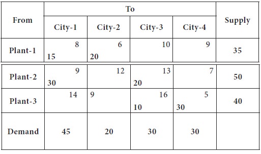
To understand the MODI Method, let us consider the solution obtained by Least Cost Method.
Step1
Step2
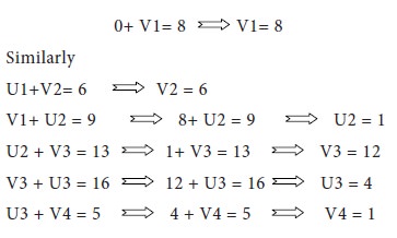
For each row, we assign ui and for each column, we will assign vj
Let us assume any one of the ui or vj as zero; preferably a row or column having maximum number of basic cells
Since there is a tie, we break it arbitrarily.
Let us assume, U1= 0
We know that U1+V1= 8 [ui+vj= Cij for all the basic cells]
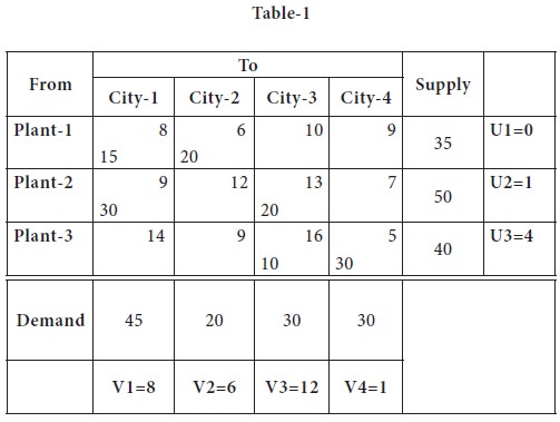
These findings are incorporated in the following table
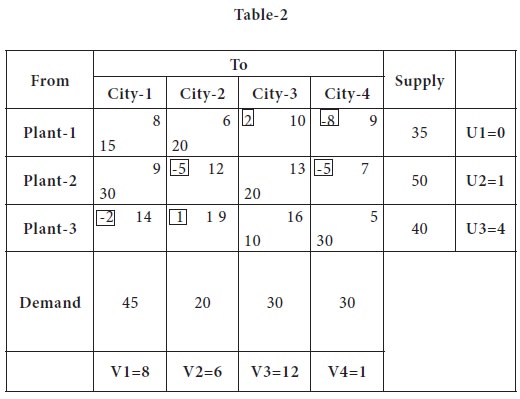
Step3
Let us compute the opportunity cost, for those cells, which are not allocated for any goods to be transported [known as non-basic cells], using (ui + vj) - Cij
For example, cell (1, 3)
Net evaluation for cell (1, 3)
= ui+vj-Cij = u1+v3-C13 = [0 + 12-10] = 2
Step4
Since all the net evaluation / opportunity costs are not negative, it is an indication of the solution is not in the optimum stage; it can be improved
Among the positive entries, the maximum positive appears in the cell (1, 3), which is 2. So this cell to be converted as a basic cell.
Step5
1. After identifying the entering variable Xrs, form a loop; this loop starts at the non-basic cell (r, s) connecting only basic cells.
2. Assign alternate plus and minus signs at the unoccupied cells on the corner points of the closed path with a plus sign at the cell being evaluated
3. Determine the maximum number of units that should be shipped to this unoccupied cell.
4. The smallest value with a negative position on the closed path indicates the number of units that can be shipped to the entering cell.
5. Now, add this quantity to all the cells on the corner points of the closed path marked with plus signs, and subtract it from those cells marked with minus signs.
6. In this way, an unoccupied cell becomes an occupied cell.
Other basic cells, the quantity allocated are modified, in such a way that without affecting the row availability and column / market requirements. The loop formed is shown below;
In the loop, between the cells with negative sign, lowest quantity allocated is 15, in the cell (1, 1); it should be shifted to the cell (1, 3), where there is a positive sign.
Thus, wherever there is a positive sign, the quantity is added; in the negative signed cell, it is subtracted.
Also, when we move the quantities, we should not move to 3 cells in a row or column; the movement of goods will be always in terms of even numbers.
You may notice in the above table, while moving the goods, we skipped the basic cell (1, 2) from the loop. Other allocations remain as such; we will now compute the cost of this allocation.
The total transportation cost
= (20 X 6) + (15 X 10) + (45 X 9) + (5 X 13) + (10 X 16) + (30 X 5)
= 120 + 150 + 405 + 65 + 160 + 150
= 1050
You may note that Least Cost method which has an initial cost of allocation as 1080, reduced by Rupees 30 by MODI / u-v method.
Once again, we check, whether the solution is optimum or not; we start again to compute the ui and vj for each row and column;
We assume V3 = 0, since it has 3 basic cells in the column and repeat the same process.
Now we will compute the Net evaluation / opportunity cost for the non-basic cells and try to form the loop, if there are positive opportunity cost in any of the cells.
The maximum positive appears in the cell (3, 2); it should be converted as basic cell and the loop is shown in the above table. The modified distribution is shown below and the cost is computed.
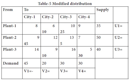
You may note that the cost of
allocation is
=(10X 6) + (25X 10) + (45 X 9) + (5 X 13) + (10 X 9) + (30 X 5)
= 60 + 250 + 405 + 65 + 90 + 150
= 1020
Since, the net evaluation / opportunity cost is negative for all the non-basic cells, it is indication that the solution is in the optimum stage.
Unbalanced Transportation Models: If the demand is not equal to supply, the transportation problems are known as unbalanced transportation problems.
You have to add a dummy row / column with zero as transportation cost with the shortfall (difference between supply and demand) as the quantity available in the origin or marketing requirements.
Then, in the usual manner, using any one of the initial solution methods will be applied and initial solution will be obtained.
You would have noticed that the initial basic feasible solution obtained by various methods provide different starting solution. Once you obtain the initial solution by any of the method, the next step is to check the optimality of the solution obtained and if not, improve the solution and obtain the optimal solution. Two popularly known methods are ‘Stepping Stone Method’ and ‘MODI Method or u-v method.
In the stepping stone method, we have to draw as many closed paths as equal to the unoccupied cells for their evaluation. To the contrary, in MODI method, only closed path for the unoccupied cell with highest opportunity cost is drawn. Here, we will discuss only the MODI Method, which is more scientific and approaches the optimal solution faster.
Modi [Modified Distribution Method] Method - Step-by-step procedure
Step1
Determine an initial basic feasible solution using any one of the three methods:
Matrix Minimum Method
Vogel Approximation Method
Step2
Each row, assign one ‘dual’ variable, say- u1, u2, u3…; for each column, assign on dual variable – say, v1, v2, v3…
Now using the basic cells [which are assigned through any one of the three methods], and the transportation costs of those basic cells -Cij, we will determine the values of these ui and vj.
Step3
Compute the opportunity cost, for those cells, which are not allocated for any goods to be transported [known as non-basic cells], using (ui + vj) - Cij
Step4
1. Check the sign of each opportunity cost.
2. If the opportunity costs of all these unoccupied cells / non-basic cells are either negative or zero, the given solution is the optimal solution.
Step5
1. Select the unoccupied cell with the highest positive opportunity cost as the cell to be included in the next solution.
Step6
Draw a closed path or loop for the unoccupied cell selected in the previous step. A loop in a transportation table is a collection of basic cells and the cell, which is to be converted as basic cell. It is formed in such a way that, it has only even number cells in any row or column.
1. After
identifying the entering variable Xrs, form a loop; this loop starts
at the non-basic cell (r, s) connecting only basic cells.
2. Assign alternate plus and minus signs at the unoccupied cells on the corner points of the closed path with a plus sign at the cell being evaluated
3. Determine the maximum number of units that should be shipped to this unoccupied cell.
4. The smallest value with a negative position on the closed path indicates the number of units that can be shipped to the entering cell.
6. In this way, an unoccupied cell becomes an occupied cell.
7. Other basic cells, the quantity allocated are modified, in such a way that without affecting the row availability and column / market requirements
8. Such a closed path exists and is unique for any non-degenerate solution.
Please note that the right angle turn in this path is permitted only at occupied cells and at the original unoccupied cell.
Step7
Repeat the whole procedure until an optimal solution is obtained.
----------------------
To understand the MODI Method, let us consider the solution obtained by Least Cost Method.
Step1
Step2
For each row, we assign ui and for each column, we will assign vj
Let us assume any one of the ui or vj as zero; preferably a row or column having maximum number of basic cells
Since there is a tie, we break it arbitrarily.
Let us assume, U1= 0
We know that U1+V1= 8 [ui+vj= Cij for all the basic cells]
These findings are incorporated in the following table
Step3
Let us compute the opportunity cost, for those cells, which are not allocated for any goods to be transported [known as non-basic cells], using (ui + vj) - Cij
For example, cell (1, 3)
Net evaluation for cell (1, 3)
= ui+vj-Cij = u1+v3-C13 = [0 + 12-10] = 2
Net evaluation for cell (1, 4)
= ui+vj-Cij = u1+v4-C14 = [0 + 1-9] = -8
Similarly for all other cells, the net evaluation / opportunity cost is computed and placed in left hand top corner of each non-basic cell; the table is placed below;
= ui+vj-Cij = u1+v4-C14 = [0 + 1-9] = -8
Similarly for all other cells, the net evaluation / opportunity cost is computed and placed in left hand top corner of each non-basic cell; the table is placed below;
Step4
Since all the net evaluation / opportunity costs are not negative, it is an indication of the solution is not in the optimum stage; it can be improved
Among the positive entries, the maximum positive appears in the cell (1, 3), which is 2. So this cell to be converted as a basic cell.
Step5
1. After identifying the entering variable Xrs, form a loop; this loop starts at the non-basic cell (r, s) connecting only basic cells.
2. Assign alternate plus and minus signs at the unoccupied cells on the corner points of the closed path with a plus sign at the cell being evaluated
3. Determine the maximum number of units that should be shipped to this unoccupied cell.
4. The smallest value with a negative position on the closed path indicates the number of units that can be shipped to the entering cell.
5. Now, add this quantity to all the cells on the corner points of the closed path marked with plus signs, and subtract it from those cells marked with minus signs.
6. In this way, an unoccupied cell becomes an occupied cell.
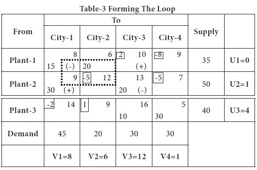
Other basic cells, the quantity allocated are modified, in such a way that without affecting the row availability and column / market requirements. The loop formed is shown below;
In the loop, between the cells with negative sign, lowest quantity allocated is 15, in the cell (1, 1); it should be shifted to the cell (1, 3), where there is a positive sign.
Thus, wherever there is a positive sign, the quantity is added; in the negative signed cell, it is subtracted.
Also, when we move the quantities, we should not move to 3 cells in a row or column; the movement of goods will be always in terms of even numbers.
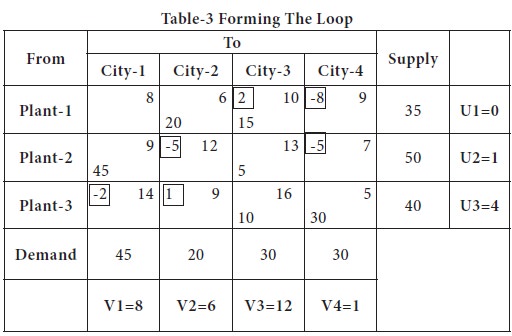
You may notice in the above table, while moving the goods, we skipped the basic cell (1, 2) from the loop. Other allocations remain as such; we will now compute the cost of this allocation.
Now the allocations are: | |
X12 = 20 | X23= 5 |
X13 = 15 | X33 = 10 |
X21 = 45 | X34 = 30 |
= (20 X 6) + (15 X 10) + (45 X 9) + (5 X 13) + (10 X 16) + (30 X 5)
= 120 + 150 + 405 + 65 + 160 + 150
= 1050
You may note that Least Cost method which has an initial cost of allocation as 1080, reduced by Rupees 30 by MODI / u-v method.
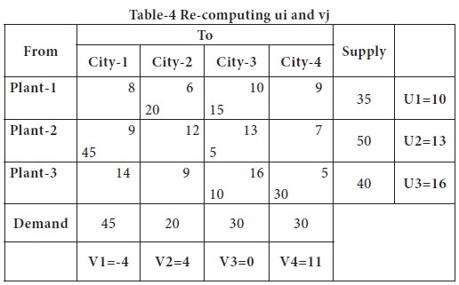
Once again, we check, whether the solution is optimum or not; we start again to compute the ui and vj for each row and column;
We assume V3 = 0, since it has 3 basic cells in the column and repeat the same process.
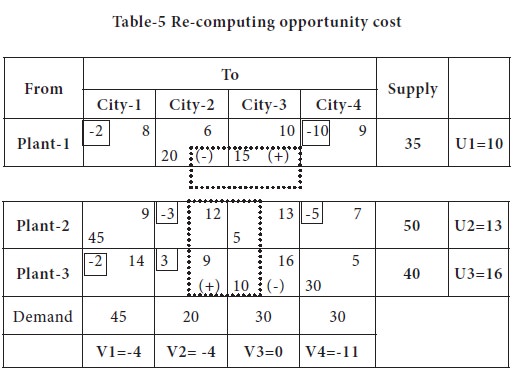
Now we will compute the Net evaluation / opportunity cost for the non-basic cells and try to form the loop, if there are positive opportunity cost in any of the cells.
The maximum positive appears in the cell (3, 2); it should be converted as basic cell and the loop is shown in the above table. The modified distribution is shown below and the cost is computed.
=(10X 6) + (25X 10) + (45 X 9) + (5 X 13) + (10 X 9) + (30 X 5)
= 60 + 250 + 405 + 65 + 90 + 150
= 1020
Thus, the total cost is reduced by modifying the
distribution / allocations made earlier. Now once again, we will check whether
the solution is optimum or not.
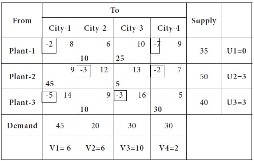
Table-6 Finding ui / vj and checking optimality of the solution
Table-6 Finding ui / vj and checking optimality of the solution
Since, the net evaluation / opportunity cost is negative for all the non-basic cells, it is indication that the solution is in the optimum stage.
Variations in the Transportation Models
Unbalanced Transportation Models: If the demand is not equal to supply, the transportation problems are known as unbalanced transportation problems.
You have to add a dummy row / column with zero as transportation cost with the shortfall (difference between supply and demand) as the quantity available in the origin or marketing requirements.
Then, in the usual manner, using any one of the initial solution methods will be applied and initial solution will be obtained.
Tags : Operations Management - Transportation / Assignment & Inventory Management
Last 30 days 2238 views