Variations in Assignment Problem- Case 1: Maximization Models - Assignment Problems

Even though the assignment algorithm is primarily a minimization model, it can be suitably modified and used for maximization models also; whenever the objective of the firm / decision maker is to maximize the return of the allocation, you have to modify the problem in the initial table and use the same Hungarian Algorithm to solve. We will solve one example here.

Variations in Assignment Problem- Case 1: Maximization Models

 

 

Even though the assignment algorithm is primarily a minimization model, it can be suitably modified and used for maximization models also; whenever the objective of the firm / decision maker is to maximize the return of the allocation, you have to modify the problem in the initial table and use the same Hungarian Algorithm to solve. We will solve one example here.

 

Example-1

 

 

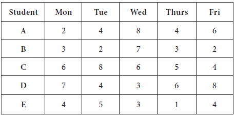
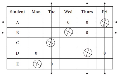
The student internship director needs as much coverage as possible in the office next week. The more hours that can be put in each day, the better. She has asked the students to provide a list of how many hours they are available each day of the week. Each student can be there on only one day and there must be a student in the office each day of the week. Use the table below and the tables provided to determine the schedule that gives the most coverage. [Note that the objective of this problem is to maximize the hours worked, not minimize].

Solution

 

As you know, the Hungarian Algorithm is primarily developed to handle minimization models; we need to modify the given problem as an ‘equivalent’ minimization model. We will convert the given problem as a minimization model in the following steps.

 

1. You have to identify the largest number in the entire matrix / table – [which is 8]

 

2. Subtract all the entries from this highest number-8 and write down the new reduced table.

 

3. This reduced table is in the form of ‘opportunity time’ of not allocating a day to a student; thus, the aim of the problem, which is in the new-reduced format, after subtracting all the entries from the highest, can be viewed as a minimization model.

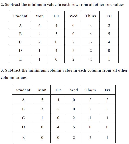
4. Then the Hungarian method is applied, which is given in the following steps.

 

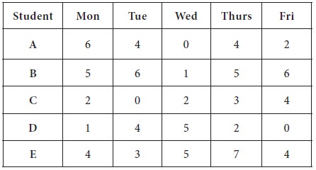
1. Convert to a minimization problem by subtracting each value from 8

4.   Now conduct the line test: draw minimum number of straight lines to cover all the zeros

 

1.  The first line is drawn at Row-4, which is having maximum number zeros (3 zeros are there in the row)

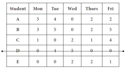
2.  The second line is drawn at Row-5, which is having maximum number zeros after removing Row-4 from further consideration (2 zeros are there in the row)

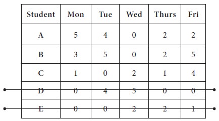
3.  Now the third line is drawn at Column-3, which is having maximum number zeros after removing Row-3, Row-4 from further consideration (2 zeros are there in the column)

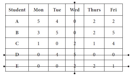
The last line is drawn at Row-3 / Column-2; you may draw the line in any manner; here, we consider the Row-3

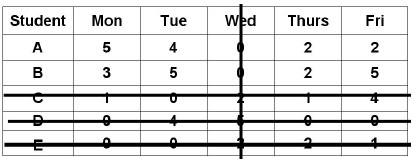
Since, the number of straight lines=4, which is less than the number of row=5, it is an indication of sufficient number of zeros are not available in the last table to do the optimum allocation. Thus, we do the following steps, in the last table obtained.

 

1. Subtract the smallest uncovered number, which is here, 2 in the above table, [not covered by any straight lines] from every uncovered number in the table.

2. We have to add this two to the numbers at intersections of covering lines; and should not make any changes for those numbers which are covered by straight lines but not crossed out by lines.

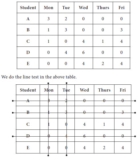
3. By doing so, we get the following table.

We now proceed to make optimum allocation with available zero entries; in the new matrix, jot down all the zeros in their respective positions.

 

1. The first unique zero is found in Row-3 and it is marked; then the column-2 is strike out;

2. The next unique zero is found in row-5 and marked; column-1 is removed

3. Since, there is no unique zero in any row or any column, you may randomly assign any zero as allocation; we allocate randomly Row-1 to Column-5. The Row-1 to Column-5 is removed from further considerations

4. Again doing, row search, unique zeros are found in Row-2 and Row-4 and marked. Thus, optimum allocation is arrived.

 

Third unique zero was found again in the row search at row-1; fourth unique zero was found at row-3 and finally the last unique zero was found in row-4.

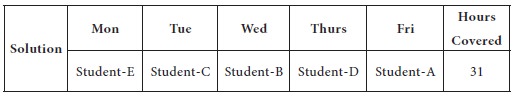
Thus, the optimum allocation is made by taking the times from original table.

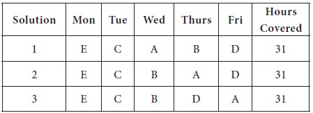
While selecting third allocation, there was no unique zero, we randomly broken the tie; so there is a possibility of more than one solution. If you choose some other zero, you may get different allocation, but the total hours will be the same as 31. You may try and check the answers, which is given below.