Operations Management - Transportation / Assignment & Inventory Management
Problem Formulation -Example - Transportation Problem
Consider the following example: Adani Power Limited, which is a electric power producing company in India, has three electric power plants that supply the needs of four cities. Each power plant can supply the following numbers of kWhr of electricity: Plant 1 – 35 million; Plant 2 – 50 million; Plant 3 – 40 million.
Consider the following example: Adani Power Limited, which is a electric power producing company in India, has three electric power plants that supply the needs of four cities. Each power plant can supply the following numbers of kWhr of electricity: Plant 1 – 35 million; Plant 2 – 50 million; Plant 3 – 40 million.
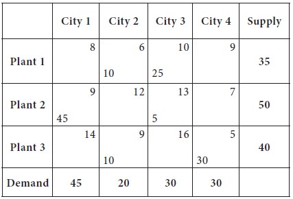
The peak power demands in these cities, which occur at the same time, are as follows (in kWhr): City 1 – 45 million; City 2 – 20 million; City 3 – 30 million; City 4 – 30 million. The costs of sending 1 million kWhr of electricity from plant to city depend on the distance the electricity must travel (see Table).
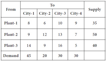
Formulate this problem to minimize the cost of meeting each city’s peak power demand.
Solution
We begin by defining a variable for each decision that Adani Power has to make.
We define, (for i = 1, 2, 3 and j = 1, 2, 3, 4)
Xij = number of (million) kWhr produced at plant i and sent to city j
Then, the objective of the Adani Power is to minimize the total transmission cost; this is achieved by allocating appropriately by linking the plant and city through the lowest cost of transmission.
As we have discussed in the Mathematical Modelling of Problems, in the Unit-2, we derive the following objective function;
Min Z = 8X11 + 6X12 + 10X13 + 9X14 + 9X21 + 12X22 + 13X23 + 7X24 + 14X31 + 9X32 + 16X33 + 5X34
This objective can be realized subject to the following constraints.
X11 + X12 + X13 + X14 ≤ 35 | ------ | (Supply
constraint from Plant-1) | ||
X21 + X22 + X23 + X24 ≤ 50 | ------ | (Supply
constraint from Plant-2) | ||
X31 + X32 + X33 + X34 ≤ 40 | ------ | (Supply
constraint from Plant-3) | ||
X11 | + X21 | + X31 ≥ 45 ----- (Demand
constraint at the city-1) | ||
X12 | + X22 | + X32 ≥ 20 | ----- | (Demand
constraint at the city-2) |
X13 + X23 + X33 ≥ 30 | ----- | (Demand
constraint at the city-3) | ||
X14 + X24 + X34 ≥ 30 | ----- | (Demand
constraint at the city-4) | ||
And obviously, Xij ≥ 0 | ||||
1. A set of ‘m’ supply points from which a good is shipped. Supply point ‘i’ can supply, at most, Si units (in the above situation, m =3, S1 = 35, S2 = 50, S3 = 40)
2. A set of ‘n’ demand points to which the good is shipped. Demand point ‘j’ must receive at least dj units of the shipped goods (you can see above, n = 4; d1 = 45, d2 = 20, d3 = 30, d4 = 30).
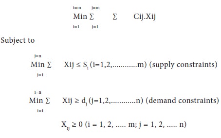
Let Xij = number of units shipped from supply point i to demand point j.
Thus, a general formulation is:
As we mentioned earlier, if ∑ Si = ∑ dj; that is supply equal demand, it is said to be balanced transportation problem. Adani issue is a balanced transportation problem.
Thus, for a balanced transportation problem,

Solution of balanced transportation problem is simpler, therefore, it is desirable to formulate a transportation problem as a balanced transportation problem.
Thus, a transportation problem is specified by the supply, the demand, and the shipping costs, so the relevant data can be summarized in a transportation tableau. The cell in row i and column j corresponds to the variable Xij.