


Home | ARTS | Operations Management
|
Initial Basic Feasible Solution - Matrix-Minima / Least Cost Method - Transportation Problem
Operations Management - Transportation / Assignment & Inventory Management
Initial Basic Feasible Solution - Matrix-Minima / Least Cost Method - Transportation Problem
Posted On :
Matrix minimum (Least cost) method is a method for computing a basic feasible solution of a transportation problem, where the basic variables are chosen on the basis of lowest unit cost of transportation.
Initial
Basic Feasible Solution - Matrix-Minima / Least Cost Method
Matrix minimum (Least cost) method is a method for computing a basic feasible solution of a transportation problem, where the basic variables are chosen on the basis of lowest unit cost of transportation. This method is very useful because it reduces the computation and the time required to determine the optimal solution. The following steps summarize the approach
Matrix-Minima / Least Cost Method: – Step-by-step procedure
1. In this method, we begin allocation by considering the minimum cost of transportation. Find the cell /variable with the smallest transportation cost (say Cij).
2. Then assign Xij its largest possible value, minimum {si, dj}.
3. Cross out row i or column j and reduce the supply or demand of the
4. Then choose from the cells that do not lie in a crossed out row or column the cell with the minimum cost and repeat procedure.
5. Continue until there is one cell that can be chosen.
For our better understanding of the method, we solve the same Adani Power limited problem which introduced and solved by North-west corner method.
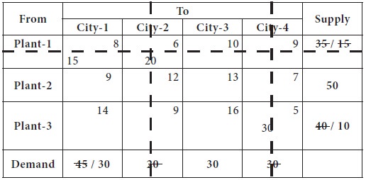
The lowest transportation cost among all the costs, is found in the cell-(3, 4), which is 5; the city requirement is 30 and plant-3 can supply at most 40.
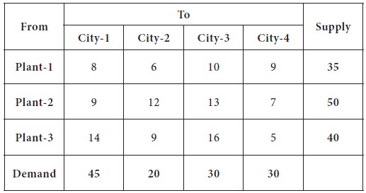
So we decide the supply the
entire 30 to city-4 from plant-3.
Now, the plant-3 can supply only 10 units to any cities and the demand for city-4 is completely exhausted. This is given in the following table.
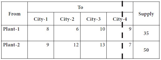
Now the lowest transportation cost among all the
costs, after removing the column-4 from consideration is found in the cell-(1,
2), which is 6; the city-2 requirement is 20 and plant-1 can supply at most 35. So we
decide the supply the entire 20 to city-2 from plant-1. Now, the plant-1 can
supply only 25 units to any cities and the demand for city-2 is completely
exhausted.
This is given in the following table.
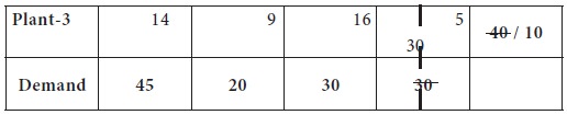
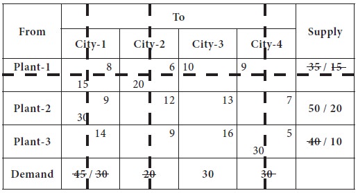
Now the lowest transportation cost among all the costs, after removing the column-2 from consideration is found in the cell-(1, 1), which is 8; the city-1 requirement is 45 and plant-1 can supply at most 15. So we decide the supply the entire 15 to city-1 from plant-1. Now, the plant-1 is completely exhausted its availability and removed from further consideration; city-1 requirement is reduced to 30.
This is given in the following table.
Now the lowest transportation cost among all the costs, after removing the row-1 from consideration is found in the cell-(2, 1), which is 9; the plant-2 can supply at most 50 and the city-1requirement is 30. So we decide the supply the entire 30 to city-1 from plant-2. Now, the plant-2 availability is reduced to 20 and the city-1 is supplied completely the need. This is given in the following table.
Now we left out with only one column, city-3, which needs 30 units; it
is supplied from plant-2 [20 units] and plant-3 [10 units].
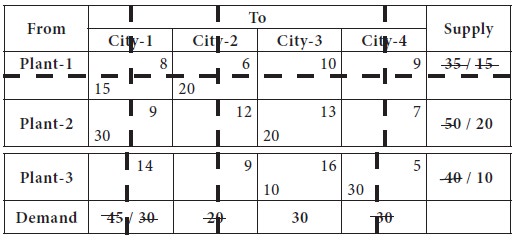
Thus, we made allocation by considering the lowest
cost in the cost matrix. The initial basic feasible solution is given below;
X11 = 15; X12= 20; X21= 30; X23= 20 X33= 10; X34= 30
Total transportation cost through the least cost / matrix minima method
Matrix minimum (Least cost) method is a method for computing a basic feasible solution of a transportation problem, where the basic variables are chosen on the basis of lowest unit cost of transportation. This method is very useful because it reduces the computation and the time required to determine the optimal solution. The following steps summarize the approach
Matrix-Minima / Least Cost Method: – Step-by-step procedure
1. In this method, we begin allocation by considering the minimum cost of transportation. Find the cell /variable with the smallest transportation cost (say Cij).
2. Then assign Xij its largest possible value, minimum {si, dj}.
3. Cross out row i or column j and reduce the supply or demand of the
4. Then choose from the cells that do not lie in a crossed out row or column the cell with the minimum cost and repeat procedure.
5. Continue until there is one cell that can be chosen.
For our better understanding of the method, we solve the same Adani Power limited problem which introduced and solved by North-west corner method.
The lowest transportation cost among all the costs, is found in the cell-(3, 4), which is 5; the city requirement is 30 and plant-3 can supply at most 40.
Now, the plant-3 can supply only 10 units to any cities and the demand for city-4 is completely exhausted. This is given in the following table.
This is given in the following table.
Now the lowest transportation cost among all the costs, after removing the column-2 from consideration is found in the cell-(1, 1), which is 8; the city-1 requirement is 45 and plant-1 can supply at most 15. So we decide the supply the entire 15 to city-1 from plant-1. Now, the plant-1 is completely exhausted its availability and removed from further consideration; city-1 requirement is reduced to 30.
This is given in the following table.
Now the lowest transportation cost among all the costs, after removing the row-1 from consideration is found in the cell-(2, 1), which is 9; the plant-2 can supply at most 50 and the city-1requirement is 30. So we decide the supply the entire 30 to city-1 from plant-2. Now, the plant-2 availability is reduced to 20 and the city-1 is supplied completely the need. This is given in the following table.
X11 = 15; X12= 20; X21= 30; X23= 20 X33= 10; X34= 30
Total transportation cost through the least cost / matrix minima method
TC = (15 X 8)
+ (20 X 6) + (30 X 9) + (20 X 13) + (10 X 16) + (30 X 5)
= 120 + 120 + 270 + 260 + 160 + 150
= 1080
You can note that the total cost of allocation through the North West corner method is 1180, whereas the cost of allocation through least cost method is 1080, which is a superior basic feasible solution than a solution obtained through north-west corner method.
Note: You may note that the number of basic cells in any transportation problem should be equal to (row+column-1).
Tags : Operations Management - Transportation / Assignment & Inventory Management
Last 30 days 6219 views