


Home | ARTS | Operations Management
|
Initial Basic Feasible Solution – Vogel’s Approximation Method [Vam] - Transportation Problem
Operations Management - Transportation / Assignment & Inventory Management
Initial Basic Feasible Solution – Vogel’s Approximation Method [Vam] - Transportation Problem
Posted On :
The Vogel Approximation Method [VAM] is an iterative procedure for computing an initial basic feasible solution of a transportation problem.
Initial
Basic Feasible Solution – Vogel’s Approximation Method [Vam]
The Vogel Approximation Method [VAM] is an iterative procedure for computing an initial basic feasible solution of a transportation problem. This method is preferred over the two methods discussed in the previous sections, because the initial basic feasible solution obtained by this method is either optimal or very nearer to the optimal solution. Therefore the amount of time required to arrive at the optimum solution is greatly reduced.
Step 1
Compute a penalty for each row in the transportation table. The penalty for a given row is the difference between the smallest cost and the
Step 2
Compute a penalty for each column of the transportation table. Identify the cell having minimum and next to minimum transportation cost in each column and write the difference (penalty) against the corresponding column.
Step 3
1. Identify the row or column with the largest penalty; make a mark in the penalty [circle the respective penalty for future references]
2. In this identified row or column, choose the cell, which is having the lowest transportation cost
3. Allocate the maximum possible quantity to the cell having lowest cost in that row or column
• Exhaust either the supply at a particular source or satisfy demand at a warehouse.
4. If there is a tie between / among the penalties computed, select that row/column which has minimum cost.
5. If there is a tie in the minimum cost also select that row/column which will have maximum possible assignments. It will considerably reduce computational work.
6. Also, you have an option of breaking the tie between / among the penalties corresponding to two or more rows or columns by breaking the tie arbitrarily
Step 4
Reduce the row supply or the column demand by the amount assigned to the cell.
3. The maximum among all the penalties [rows as well as columns together] is marked;
• In case of a tie, you may choose the row or column that is having the lowest transportation cost cell;
4. That row
or column should be allocated first; the allocation is made to the cell, which
is having lowest transportation cost; in case of tie between cells, you can
break it arbitrarily.
In the above table, it is 4, appearing in the 3rd row; the lowest transportation cost 5 appears in the cell (3, 4).
Availability at the plant-3 is 40 units and city-4 requires 30 units; so we supply the entire 30 units from plant-3;
Now the city-4 is eliminated from further consideration and plant-3 availability is reduced to 10.
The transportation table is modified with the above changes and placed below; in that table, again the process is repeated [while doing future calculations, we will not consider costs in the column-4 anymore] and row/ column penalty-2 is computed.
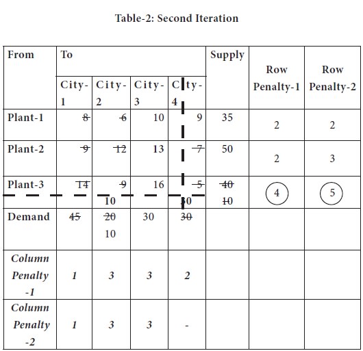
In the above table, highest penalty is 5, appearing
again in the 3rd row; the lowest transportation cost 9 appears in the cell (3,
2).
Availability at the plant-3 is 10 units and city-2 requires 20 units; so we supply the entire 10 units from plant-3;
Now the plant-3 is eliminated from further consideration and city-2 requirement is reduced to 10.
The transportation table is modified with the above changes and placed below; in that table, again the process is repeated [while doing future calculations, we will not consider costs in the column-4 & Row-3 anymore] and row/ column penalty-3 is computed.
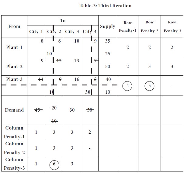
In the above table, highest penalty is 6, appearing again in the 2nd column; the lowest transportation cost 6 appears in the cell (1, 2).
Availability at the plant-1 is 35 units and city-2 requires 10 units; so we supply the entire 10 units from plant-1;
Now the city-2 is eliminated from further consideration and plant-1 requirement is reduced to 25.
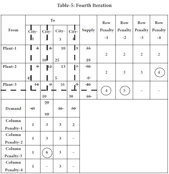
The transportation table is modified with the above changes and placed below; in that table, again the process is repeated [while doing future calculations, we will not consider costs in the column-4, column-2 & Row-3 anymore] and row/ column penalty-4 is computed.
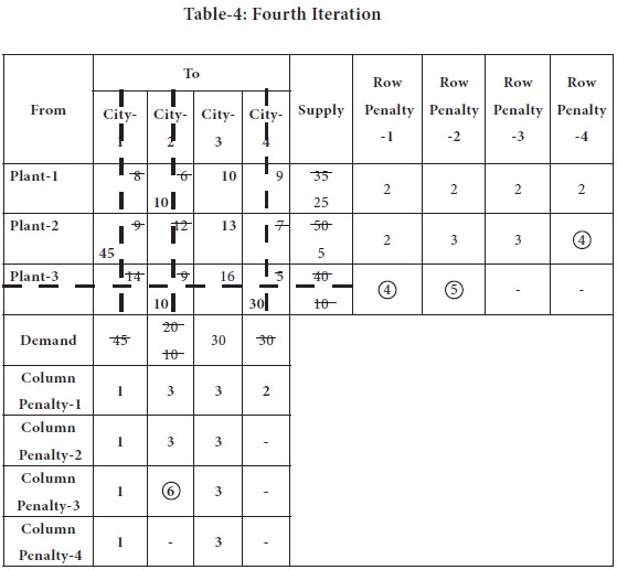
In the above table, highest penalty is 6, appearing again in the 2nd column; the lowest transportation cost 6 appears in the cell (1, 2).
Availability at the plant-1 is 35 units and city-2 requires 10 units; so we supply the entire 10 units from plant-1;
Now the city-2 is eliminated from further consideration and plant-1 requirement is reduced to 25.
Now we left out with only one column, city-3. This is serviced by plant-1, 25 units and plant-2, by 5 units.
Thus, we fulfil the requirements of all the cities and from the plants. We made the initial allocation through Vogel’s approximation method.
Now the allocations are:
The total transportation cost
= (10 X 6) + (25 X 10) + (45 X 9) + (5 X 13) + (10 X 9) + (30 X 5)
= 60 + 250 + 405 + 65 + 90 + 150
= 1020
You can note that the total cost of allocation through the North West corner method is 1180; least cost method is 1080, whereas through VAM, we get 1020, which is a superior basic feasible solution than a solution obtained through other methods.
Note: You may
note that the number of basic cells in any transportation problem should be equal to (row+column-1).
The Vogel Approximation Method [VAM] is an iterative procedure for computing an initial basic feasible solution of a transportation problem. This method is preferred over the two methods discussed in the previous sections, because the initial basic feasible solution obtained by this method is either optimal or very nearer to the optimal solution. Therefore the amount of time required to arrive at the optimum solution is greatly reduced.
Vogel’s Approximation Method [Vam]:– Step-by-step procedure
Step 1
Compute a penalty for each row in the transportation table. The penalty for a given row is the difference between the smallest cost and the
Step 2
Compute a penalty for each column of the transportation table. Identify the cell having minimum and next to minimum transportation cost in each column and write the difference (penalty) against the corresponding column.
Step 3
1. Identify the row or column with the largest penalty; make a mark in the penalty [circle the respective penalty for future references]
2. In this identified row or column, choose the cell, which is having the lowest transportation cost
3. Allocate the maximum possible quantity to the cell having lowest cost in that row or column
• Exhaust either the supply at a particular source or satisfy demand at a warehouse.
4. If there is a tie between / among the penalties computed, select that row/column which has minimum cost.
5. If there is a tie in the minimum cost also select that row/column which will have maximum possible assignments. It will considerably reduce computational work.
6. Also, you have an option of breaking the tie between / among the penalties corresponding to two or more rows or columns by breaking the tie arbitrarily
Step 4
Reduce the row supply or the column demand by the amount assigned to the cell.
Step 5
1. If the row supply is now zero, eliminate the row;
2. If the column demand is now zero, eliminate the column
3. If both the row supply and the column demand is zero, eliminate either the row or column.
4. After eliminating the row or column, in the left out row or column, enter the balance as zero [this will help in avoiding degeneracy, which is an issue while solving the problem for optimality check]
5. In future iterations, if the row or column with zero is selected, follow the same procedure, as if you are allocating a quantity; only the difference is, you will allocate zero as quantity to a cell. This will avoid number of other steps, which are slightly complicated.
Step 6
Recompute the row and column difference for the reduced transportation table, which has obtained by omitting rows or columns crossed out in the preceding step.
Step 7
Repeat the above procedure until the entire supply at factories are exhausted to satisfy demand at different warehouses.
For our better understanding of the method, we solve the same Adani Power limited problem which introduced and solved by North-west corner method as well as Least Cost Methods.
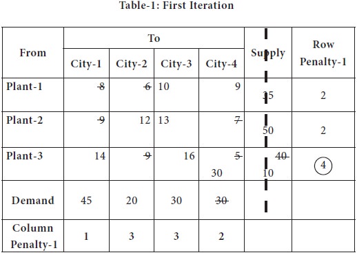
1. The lowest and next lowest for each row is located and penalty is computed and marked against the respective rows.
2. Similarly, the lowest and next lowest is located and penalty is computed for each column and marked against the respective columns.
1. If the row supply is now zero, eliminate the row;
2. If the column demand is now zero, eliminate the column
3. If both the row supply and the column demand is zero, eliminate either the row or column.
4. After eliminating the row or column, in the left out row or column, enter the balance as zero [this will help in avoiding degeneracy, which is an issue while solving the problem for optimality check]
5. In future iterations, if the row or column with zero is selected, follow the same procedure, as if you are allocating a quantity; only the difference is, you will allocate zero as quantity to a cell. This will avoid number of other steps, which are slightly complicated.
Step 6
Recompute the row and column difference for the reduced transportation table, which has obtained by omitting rows or columns crossed out in the preceding step.
Step 7
Repeat the above procedure until the entire supply at factories are exhausted to satisfy demand at different warehouses.
For our better understanding of the method, we solve the same Adani Power limited problem which introduced and solved by North-west corner method as well as Least Cost Methods.
1. The lowest and next lowest for each row is located and penalty is computed and marked against the respective rows.
2. Similarly, the lowest and next lowest is located and penalty is computed for each column and marked against the respective columns.
3. The maximum among all the penalties [rows as well as columns together] is marked;
• In case of a tie, you may choose the row or column that is having the lowest transportation cost cell;
In the above table, it is 4, appearing in the 3rd row; the lowest transportation cost 5 appears in the cell (3, 4).
Availability at the plant-3 is 40 units and city-4 requires 30 units; so we supply the entire 30 units from plant-3;
Now the city-4 is eliminated from further consideration and plant-3 availability is reduced to 10.
The transportation table is modified with the above changes and placed below; in that table, again the process is repeated [while doing future calculations, we will not consider costs in the column-4 anymore] and row/ column penalty-2 is computed.
Availability at the plant-3 is 10 units and city-2 requires 20 units; so we supply the entire 10 units from plant-3;
Now the plant-3 is eliminated from further consideration and city-2 requirement is reduced to 10.
The transportation table is modified with the above changes and placed below; in that table, again the process is repeated [while doing future calculations, we will not consider costs in the column-4 & Row-3 anymore] and row/ column penalty-3 is computed.
In the above table, highest penalty is 6, appearing again in the 2nd column; the lowest transportation cost 6 appears in the cell (1, 2).
Availability at the plant-1 is 35 units and city-2 requires 10 units; so we supply the entire 10 units from plant-1;
Now the city-2 is eliminated from further consideration and plant-1 requirement is reduced to 25.
The transportation table is modified with the above changes and placed below; in that table, again the process is repeated [while doing future calculations, we will not consider costs in the column-4, column-2 & Row-3 anymore] and row/ column penalty-4 is computed.
In the above table, highest penalty is 6, appearing again in the 2nd column; the lowest transportation cost 6 appears in the cell (1, 2).
Availability at the plant-1 is 35 units and city-2 requires 10 units; so we supply the entire 10 units from plant-1;
Now the city-2 is eliminated from further consideration and plant-1 requirement is reduced to 25.
Now we left out with only one column, city-3. This is serviced by plant-1, 25 units and plant-2, by 5 units.
Thus, we fulfil the requirements of all the cities and from the plants. We made the initial allocation through Vogel’s approximation method.
Now the allocations are:
X12 = 10 | X13= 25 |
X21 = 45 | X23 = 5 |
X32 = 10 | X34 = 30 |
= (10 X 6) + (25 X 10) + (45 X 9) + (5 X 13) + (10 X 9) + (30 X 5)
= 60 + 250 + 405 + 65 + 90 + 150
= 1020
You can note that the total cost of allocation through the North West corner method is 1180; least cost method is 1080, whereas through VAM, we get 1020, which is a superior basic feasible solution than a solution obtained through other methods.
Tags : Operations Management - Transportation / Assignment & Inventory Management
Last 30 days 2415 views