


Operations Management - Transportation / Assignment & Inventory Management
Mathematical Formulation of Transportation Problems
Posted On :
As we discussed just above, Transportation models deals with the transportation of a product manufactured at different plants or factories (supply origins) to a number of manufactured at different warehouses (demand destinations).
Mathematical Formulation of
Transportation Problems
As we discussed just above, Transportation models deals with the transportation of a product manufactured at different plants or factories (supply origins) to a number of manufactured at different warehouses (demand destinations). The objective is to satisfy the destination requirements within the plant’s capacity constraints at the minimum transportation cost. Transportation models thus typically arise in situations involving physical movement of goods from plants to warehouses, warehouses to wholesalers, wholesalers to retailers and retailers to customers. Solution of the transportation models requires the determination of how many units should be transported from each supply origin to each demands destination in order to satisfy all the destination demands white minim sing the total associated cost of transportation
Consider a soft drink manufacturing firm, which has m plants located in m different cities. The total production is to be supplied to the retail shops in ‘n’ different cities. We want to determine the transportation schedule that minimizes the total cost of transporting soft drinks from various plants to various retail shops. This situation can be formulated as a linear programming problem.
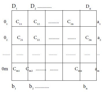
Let us consider the m-plant locations (origins) as O1, O2… Om and the n-retail markets (destination) as D1, D2… Dn respectively. Let ai ≥ 0, i= 1, 2 ….m, be the amount available at the ith plant-Oi. Let the
amount required at the jth market-Dj be bj ≥ 0, j= 1,2,….n.
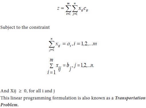
Let the cost of transporting one unit of soft drink form ith origin to jth destination be Cij, i= 1, 2 ….m, j=1, 2….n. If Xij ≥ 0 be the amount of soft drink to be transported from ith origin to jth destination then the problem is to determine xij so as to Minimize the total cost of transportation, which is denoted as Z.
The above set of constraints represents ‘m+n’ equations in m X n non-negative variables. Each variable Xij appears in exactly two constraints, one is associated
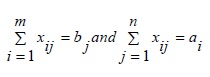
with the origin and the other is associated with the destination. It allows us to put the above LPP in the matrix form, the elements of A are either 0 or 1.
Requirement
A basic assumption is that the distribution costs of units from source i to destination j is directly proportional to the number of units distributed.
Moreover, if the demand is equal to supply in a given transportation model, it is called as a balanced problem; in a balanced problem all the products that can be supplied are used to meet the demand. There are no slacks and so all constraints are equalities rather than inequalities.
On the other hand, if the demand is not equal to supply, it is known as unbalanced transportation model. However, to obtain an initial solution, we have to modify the unbalanced transportation
For many applications, the supply and demand quantities in the model will have integer values and implementation will require that the distribution quantities also be integers. Fortunately, the unit coefficients of the unknown variables in the constraints guarantee an optimal solution with only integer values.
As we discussed just above, Transportation models deals with the transportation of a product manufactured at different plants or factories (supply origins) to a number of manufactured at different warehouses (demand destinations). The objective is to satisfy the destination requirements within the plant’s capacity constraints at the minimum transportation cost. Transportation models thus typically arise in situations involving physical movement of goods from plants to warehouses, warehouses to wholesalers, wholesalers to retailers and retailers to customers. Solution of the transportation models requires the determination of how many units should be transported from each supply origin to each demands destination in order to satisfy all the destination demands white minim sing the total associated cost of transportation
Consider a soft drink manufacturing firm, which has m plants located in m different cities. The total production is to be supplied to the retail shops in ‘n’ different cities. We want to determine the transportation schedule that minimizes the total cost of transporting soft drinks from various plants to various retail shops. This situation can be formulated as a linear programming problem.
Let us consider the m-plant locations (origins) as O1, O2… Om and the n-retail markets (destination) as D1, D2… Dn respectively. Let ai ≥ 0, i= 1, 2 ….m, be the amount available at the ith plant-Oi. Let the
amount required at the jth market-Dj be bj ≥ 0, j= 1,2,….n.
Let the cost of transporting one unit of soft drink form ith origin to jth destination be Cij, i= 1, 2 ….m, j=1, 2….n. If Xij ≥ 0 be the amount of soft drink to be transported from ith origin to jth destination then the problem is to determine xij so as to Minimize the total cost of transportation, which is denoted as Z.
The Transportation Table
The above set of constraints represents ‘m+n’ equations in m X n non-negative variables. Each variable Xij appears in exactly two constraints, one is associated
with the origin and the other is associated with the destination. It allows us to put the above LPP in the matrix form, the elements of A are either 0 or 1.
Requirement
Assumptions in Transportation Problems
A basic assumption is that the distribution costs of units from source i to destination j is directly proportional to the number of units distributed.
Moreover, if the demand is equal to supply in a given transportation model, it is called as a balanced problem; in a balanced problem all the products that can be supplied are used to meet the demand. There are no slacks and so all constraints are equalities rather than inequalities.
On the other hand, if the demand is not equal to supply, it is known as unbalanced transportation model. However, to obtain an initial solution, we have to modify the unbalanced transportation
For many applications, the supply and demand quantities in the model will have integer values and implementation will require that the distribution quantities also be integers. Fortunately, the unit coefficients of the unknown variables in the constraints guarantee an optimal solution with only integer values.
Tags : Operations Management - Transportation / Assignment & Inventory Management
Last 30 days 14814 views