


Home | ARTS | Operations Management
|
Properties of The Simplex Method - Linear Programming – Problem Solving [SIMPLEX METHOD]
Operations Management - Introduction to Operations Research
Properties of The Simplex Method - Linear Programming – Problem Solving [SIMPLEX METHOD]
Posted On :
If an artificial variable is in an optimal solution of the equivalent model at a nonzero level, then no feasible solution for the original model exists. On the contrary, if the optimal solution of the equivalent model does not contain an artificial variable at a non-zero level, the solution is also optimal for the original model.
Properties of The Simplex
Method
1. The Simplex method for maximizing the objective function starts at a basic feasible solution for the equivalent model and moves to an adjacent basic feasible solution that does not decrease the value of the objective function. If such a solution does not exist, an optimal
2. If an artificial variable is in an optimal solution of the equivalent model at a nonzero level, then no feasible solution for the original model exists. On the contrary, if the optimal solution of the equivalent model does not contain an artificial variable at a non-zero level, the solution is also optimal for the original model.
3. If all the slack, surplus, and artificial variables are zero when an optimal solution of the equivalent model is reached, then all of the constraints in the original model are strict “equalities” for the values of the variables that optimize the objective function.
4. If a non-basic variable has zero coefficients in the objective function equation when an optimal solution is reached, there are multiple optimal solutions. In fact, there is infinity of optimal solutions, the Simplex method finds only one optimal solution and stops.
5. Once an artificial variable leaves the set of basic variables (the basis), it will never enter the basis again, so all calculations for that variable can be ignored in future steps.
6. When selecting the variable to leave the current basis:
(a) If two or more ratios are smallest, choose one arbitrarily.
(b) If a positive ratio does not exist, the objective function in the original model is not bounded by the constraints. Thus a Finite optimal solution for The original model does not exist.
7. If a basis has a variable at zero level, it is called a degenerate basis.
8. Although cycling is possible, there have never been any practical problems for which the Simplex method failed to converge.
Step 2
An obvious initial basic feasible solution is given by XB=B-1b.
Where B=I3 and XB=[X3 X4 X5], & I3 stands for Identity matrix of order of 3 (that is a 3X3 matrix). That is,
[X3 X4 X5] = I3 [8 12 3] = [8 12 3]
From the starting tableau, it is apparent that there are two Zj-Cj values, which are having negative coefficients.
We choose the most negative of these, viz., -2. The corresponding column vector y2, therefore, enters the basis.
Since, all Zj-Cj>=0, we conclude that there is no more improvement possible and the problem is in its optimum stage.
Therefore, the optimal solution for the given problem is
X1= 2 X2= 5 Max Z = 12
Example-2
Solve the following problem by simplex method [the same problem is solved under graphical method already]
Maximize z = 15X1 + 10X2
Subject to constraints
4X1+6X2 <=360
3X1+0X2<=180
0X1+5X2 <=200
X1, X2>=0
Solution
The problem is converted into standard form by adding slack variables X3, X4 & X5 to the each of the constraint.
4X1+6X2 +X3=360
3X1+0X2+X4=180
0X1+5X2+X5=200
And the modified objective function is
Maximize z = 15X1 + 10X2 +0X3 + 0X4 + 0X5
Then the first simplex table is arrived.
Then we will compute the Zj-Cj (net evaluations) for each column as follows;
For the first column Y1, it is computed as follows; Z1-C1= cB y1-c1
[(0*4) + (0*1) + (0* 0)]-15 = -15
In similar lines, the evaluations are calculated for all the columns and placed in the last row of the table.
Then we will compute the ratios, using RHS of each constraint and dividing it by the respective entering column non-zero, non-negative quantities; this is placed in the last column of the following table.
Then, the minimum among the value is chosen as leaving variable; therefore, X1 entering the basis and X4 leaving the basis.
Then, we need to do the simple ‘row’ operations or modified ‘Gauss-Jordon’ Elimination process. We have to have 1 at the row/column intersection [known as pivotal element] and the rest of the entries in the pivotal column as zero.
The first row is replaced by dividing all the entries by 4, which is the ‘pivotal’ element of the table [The number in the intersection of ‘entering column’ and ‘leaving row’] and placed in the second iteration table in the corresponding position of the original place. For example, consider the original first row

Now the X3=360 is replaced by the following calculation
In the next step, X2 is entering the basis and X3 leaves the basis; the row operations are carried out and the new table-3 is given below;
You can notice that in the end of second iteration, all the net evaluations (Zj-Cj) are non-negative; this implies that the current solution is in the optimal stage.
Therefore,
X1 = 60 X2= 20 Max Z=(15* 60) + (10 * 20) = 900+200=1100 You can recall that the same answer was obtained through the graphical method.
In the next sections, we solve the special cases, attempted by graphical method.
1. The Simplex method for maximizing the objective function starts at a basic feasible solution for the equivalent model and moves to an adjacent basic feasible solution that does not decrease the value of the objective function. If such a solution does not exist, an optimal
2. If an artificial variable is in an optimal solution of the equivalent model at a nonzero level, then no feasible solution for the original model exists. On the contrary, if the optimal solution of the equivalent model does not contain an artificial variable at a non-zero level, the solution is also optimal for the original model.
3. If all the slack, surplus, and artificial variables are zero when an optimal solution of the equivalent model is reached, then all of the constraints in the original model are strict “equalities” for the values of the variables that optimize the objective function.
4. If a non-basic variable has zero coefficients in the objective function equation when an optimal solution is reached, there are multiple optimal solutions. In fact, there is infinity of optimal solutions, the Simplex method finds only one optimal solution and stops.
5. Once an artificial variable leaves the set of basic variables (the basis), it will never enter the basis again, so all calculations for that variable can be ignored in future steps.
6. When selecting the variable to leave the current basis:
(a) If two or more ratios are smallest, choose one arbitrarily.
(b) If a positive ratio does not exist, the objective function in the original model is not bounded by the constraints. Thus a Finite optimal solution for The original model does not exist.
7. If a basis has a variable at zero level, it is called a degenerate basis.
8. Although cycling is possible, there have never been any practical problems for which the Simplex method failed to converge.
Example
Maximize z = X1+2X2
Subject to:
-X1+2X2<=8,
X1+2X2<=12,
X1-X2<=3;
X1>=0 and X2>=0.
Solution
Step 1
Introducing the slack Variable X3>=0, X4>=0 and X5>=0 to the first, second and third constraints respectively and convert the problem into standard form.
-X1+2X2 + X3 = 8,
X1+2X2 +X4 =12,
X1- X2 +X5 = 3;
And the modified objective function is
Z=X1+2X2+0X3+0X4+0X5
X1, X2, X3, X4 & X5 >0
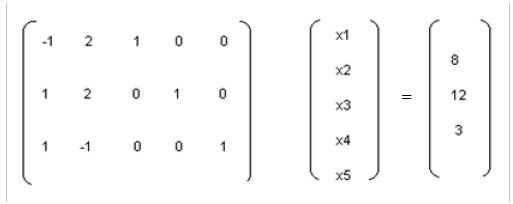
The constraints the given L.P.P are converted into the system of equations:
X1, X2, X3, X4 & X5 >0
The constraints the given L.P.P are converted into the system of equations:
Step 2
An obvious initial basic feasible solution is given by XB=B-1b.
Where B=I3 and XB=[X3 X4 X5], & I3 stands for Identity matrix of order of 3 (that is a 3X3 matrix). That is,
[X3 X4 X5] = I3 [8 12 3] = [8 12 3]
Step 3
We compute yj and the net evaluations, zj-cj corresponding to the basic variables X3, X4 and X5:
Z3-C3 = cB y3-c3 = (0 0 0) e1-0 = 0,
Z4-C4 = cB y4-c4 = (0 0 0) e2-0 = 0,
Z5-C5 = cB y5-c5 = (0 0 0) e3-0 = 0.
Step 4 - Deciding the entering variable
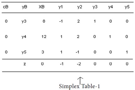
Making use of the above information, the starting simplex tableau is written as follows:
We compute yj and the net evaluations, zj-cj corresponding to the basic variables X3, X4 and X5:
y1=B-1a1 | = | I3 [-1 | 1 | 1] | = | [1 1 | 1] | |
y2=B-1a1 | = | I3 [2 | 2 | -1] | = [2 2
-1] | |||
y3 =
B-1e1 = e1, y4 = B-1e2 = e2 | and | y5 =
B-1e3 = e3. | ||||||
Z1-C1 =
cB y1-c1 = (0 0 | 0) [-1 | 1 | 1]-1 =
-1. | |||||
Z2-C2 =
cB y2-c2 = (0 0 0) [2 | 2 | -1]-2 | = -2. | |||||
Z3-C3 = cB y3-c3 = (0 0 0) e1-0 = 0,
Z4-C4 = cB y4-c4 = (0 0 0) e2-0 = 0,
Z5-C5 = cB y5-c5 = (0 0 0) e3-0 = 0.
Step 4 - Deciding the entering variable
Making use of the above information, the starting simplex tableau is written as follows:
From the starting tableau, it is apparent that there are two Zj-Cj values, which are having negative coefficients.
We choose the most negative of these, viz., -2. The corresponding column vector y2, therefore, enters the basis.
Step 5 - Deciding the leaving variable
Now, we will compute the ratios using the entering column elements and RHS of each constraint.
Each row of the table, the respective RHS coefficient of the constraint is divided by entering column, non-zero element and placed in the last column of the table. Then, the minimum among the value is chosen as leaving variable.
Min {XBi/Yi2, Yi2>0} = Min. {8/2, 12/2, no ratio for third row} = 4. Since the minimum ratio occurs for the first row, basis vector Y3 leaves the basis. The common intersection element y12 (=2) become the leading element for updating. We indicate the leading element in bold type with a star *.
Step 6
Convert the leading element y12 to unity and all other elements in its column (i.e.y2) to zero by the following transformations:
Y11 =Y11/Y12 =1/2, Y10 = Y10/Y12 =8/2 or 4, so on,
Y20=y20-(y10/y11) y22=12-(8/2) (2) =4.
Y30=y30-(y10/y12)
y32=3-(8/2) (-2) =11.
Y21=y21-(y11/y12) y22=1-(-1/2) (2) =2.
Y31=y31-(y11/y12) y32=1-(-1/2) (-2) =0. And so on………
Step 7
Using the above computations, the following iterated simplex tableau is obtained:
The above simplex tableau yields a new basic feasible solution with the increased value of z.
Now since z1-c1 < 0, y1 enters the basis.
Also, since Min. {X Bi / yi >0} = Min {4/2, 7/ (1/2)} = 2, y4 leaves the basis.
Thus the leading element will be y21 (=2).
Converting the leadwing element to unity and all other elements of yi to zero by usual row transformations the next iterated tableau is obtained.
Y31=y31-(y11/y12) y32=1-(-1/2) (-2) =0. And so on………
Step 7
Using the above computations, the following iterated simplex tableau is obtained:
The above simplex tableau yields a new basic feasible solution with the increased value of z.
Now since z1-c1 < 0, y1 enters the basis.
Also, since Min. {X Bi / yi >0} = Min {4/2, 7/ (1/2)} = 2, y4 leaves the basis.
Thus the leading element will be y21 (=2).
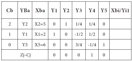
Converting the leadwing element to unity and all other elements of yi to zero by usual row transformations the next iterated tableau is obtained.
Since, all Zj-Cj>=0, we conclude that there is no more improvement possible and the problem is in its optimum stage.
Therefore, the optimal solution for the given problem is
X1= 2 X2= 5 Max Z = 12
Example-2
Solve the following problem by simplex method [the same problem is solved under graphical method already]
Maximize z = 15X1 + 10X2
Subject to constraints
4X1+6X2 <=360
3X1+0X2<=180
0X1+5X2 <=200
X1, X2>=0
Solution
The problem is converted into standard form by adding slack variables X3, X4 & X5 to the each of the constraint.
4X1+6X2 +X3=360
3X1+0X2+X4=180
0X1+5X2+X5=200
And the modified objective function is
Maximize z = 15X1 + 10X2 +0X3 + 0X4 + 0X5
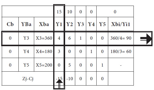
Then the first simplex table is arrived.
Then we will compute the Zj-Cj (net evaluations) for each column as follows;
For the first column Y1, it is computed as follows; Z1-C1= cB y1-c1
[(0*4) + (0*1) + (0* 0)]-15 = -15
In similar lines, the evaluations are calculated for all the columns and placed in the last row of the table.
Then we will compute the ratios, using RHS of each constraint and dividing it by the respective entering column non-zero, non-negative quantities; this is placed in the last column of the following table.
Then, the minimum among the value is chosen as leaving variable; therefore, X1 entering the basis and X4 leaving the basis.
Then, we need to do the simple ‘row’ operations or modified ‘Gauss-Jordon’ Elimination process. We have to have 1 at the row/column intersection [known as pivotal element] and the rest of the entries in the pivotal column as zero.
The first row is replaced by dividing all the entries by 4, which is the ‘pivotal’ element of the table [The number in the intersection of ‘entering column’ and ‘leaving row’] and placed in the second iteration table in the corresponding position of the original place. For example, consider the original first row
Now the X3=360 is replaced by the following calculation
New
element= Old element – [respective element in the pivotal row X respective element in the pivotal column/pivotal element]
New element for 360 = 360 – [(180 * 4) /3] = 360-240 = 120
Similarly, for the Y2 column, of the first row, for the ‘6’, the new element is arrived in similar way
New element for 6 = 6 – [(4 * 0) /3] = 6-0 = 6
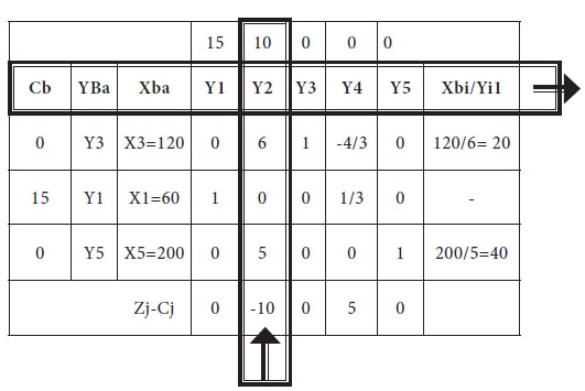
The new table-2 is arrived as follows with the following changes;
• X3 is replaced by X1
• Row operations are carried out
Table-2- which is showing the entering column vector and leaving variable
New element for 360 = 360 – [(180 * 4) /3] = 360-240 = 120
Similarly, for the Y2 column, of the first row, for the ‘6’, the new element is arrived in similar way
New element for 6 = 6 – [(4 * 0) /3] = 6-0 = 6
The new table-2 is arrived as follows with the following changes;
• X3 is replaced by X1
• Row operations are carried out
Table-2- which is showing the entering column vector and leaving variable
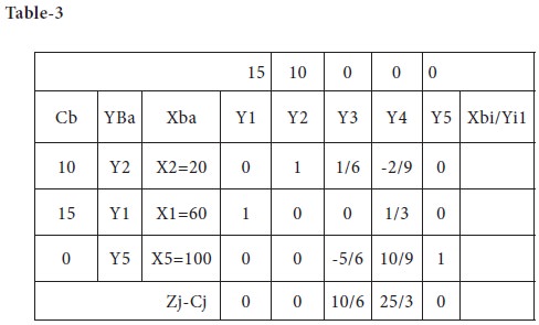
In the next step, X2 is entering the basis and X3 leaves the basis; the row operations are carried out and the new table-3 is given below;
You can notice that in the end of second iteration, all the net evaluations (Zj-Cj) are non-negative; this implies that the current solution is in the optimal stage.
Therefore,
X1 = 60 X2= 20 Max Z=(15* 60) + (10 * 20) = 900+200=1100 You can recall that the same answer was obtained through the graphical method.
In the next sections, we solve the special cases, attempted by graphical method.
Tags : Operations Management - Introduction to Operations Research
Last 30 days 3060 views