


Research Methodology - Statistical Analysis
NORMAL DISTRIBUTION - Statistical Analysis
Posted On :
The normal distribution was first described by Abraham Demoivre (1667-1754) as the limiting form of binomial model in 1733.
NORMAL DISTRIBUTION
The normal distribution was first described by Abraham Demoivre (1667-1754) as the limiting form of binomial model in 1733. Normal distribution was rediscovered by Gauss in 1809 and by Laplace in 1812. Both Gauss and Laplace were led to the distribution by their work on the theory of errors of observations arising in physical measuring processes particularly in astronomy.
The probability function of a Normal Distribution is defined as:
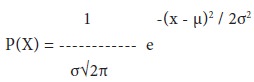
Where, X = Values of the continuous random variable, µ = Mean of the normal random variable, e = 2.7183, π = 3.1416
Binomial, Poisson and Normal Distribution are closely related to one other. When N is large while the probability P of the occurrence of an event is close to zero so that q = (1-p) the binomial distribution is very closely approximated by the Poisson distribution with m = np.
The Poisson distribution approaches a normal distribution with standardized variable (x – m)/ √m as m increases to infinity.
The important properties of the normal distribution are:-
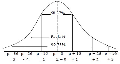
1. The normal curve is “bell shaped” and symmetrical in nature. The distribution of the frequencies on either side of the maximum ordinate of the curve is similar with each other.
2. The maximum ordinate of the normal curve is at x = µ. Hence the mean, median and mode of the normal distribution coincide.
3. It ranges between - ∞ to + ∞
4. The value of the maximum ordinate is 1/ σ√2π.
5. The points where the curve change from convex to concave or vice versa is at X = µ ± σ.
6. The first and third quartiles are equidistant from median.
7. The area under the normal curve distribution are:
a. µ ± 1σ covers 68.27% area;
b. µ ± 2σ covers 95.45% area.
c. µ ± 3σ covers 99.73% area.
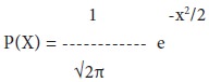
8. When µ = 0 and σ = 1, then the normal distribution will be a standard normal curve. The probability function of standard normal curve is
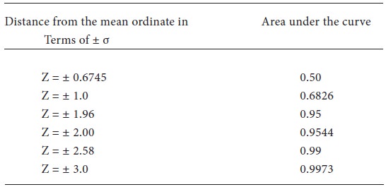
The following table gives the area under the normal probability curve for some important value of Z.
The normal distribution was first described by Abraham Demoivre (1667-1754) as the limiting form of binomial model in 1733. Normal distribution was rediscovered by Gauss in 1809 and by Laplace in 1812. Both Gauss and Laplace were led to the distribution by their work on the theory of errors of observations arising in physical measuring processes particularly in astronomy.
The probability function of a Normal Distribution is defined as:
Where, X = Values of the continuous random variable, µ = Mean of the normal random variable, e = 2.7183, π = 3.1416
Relation Between Binomial, Poisson And Normal Distributions
Binomial, Poisson and Normal Distribution are closely related to one other. When N is large while the probability P of the occurrence of an event is close to zero so that q = (1-p) the binomial distribution is very closely approximated by the Poisson distribution with m = np.
The Poisson distribution approaches a normal distribution with standardized variable (x – m)/ √m as m increases to infinity.
Normal distribution and its properties
The important properties of the normal distribution are:-
1. The normal curve is “bell shaped” and symmetrical in nature. The distribution of the frequencies on either side of the maximum ordinate of the curve is similar with each other.
2. The maximum ordinate of the normal curve is at x = µ. Hence the mean, median and mode of the normal distribution coincide.
3. It ranges between - ∞ to + ∞
4. The value of the maximum ordinate is 1/ σ√2π.
5. The points where the curve change from convex to concave or vice versa is at X = µ ± σ.
6. The first and third quartiles are equidistant from median.
7. The area under the normal curve distribution are:
a. µ ± 1σ covers 68.27% area;
b. µ ± 2σ covers 95.45% area.
c. µ ± 3σ covers 99.73% area.
8. When µ = 0 and σ = 1, then the normal distribution will be a standard normal curve. The probability function of standard normal curve is
The following table gives the area under the normal probability curve for some important value of Z.
9. All odd moments are equal to zero.
Find the probability that the standard normal value lies between 0 and 1.5
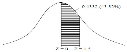
As the mean, Z = 0.
To find the area between Z = 0 and Z = 1.5, look the area between 0 and 1.5, from the table. It is 0.4332 (shaded area)
Illustration:
The results of a particular examination are given below in a summary form:
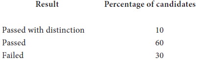
It is known that a candidate gets plucked if he obtains less than 40 marks, out of 100 while he must obtain at least 75 marks in order to pass with distinction. Determine the mean and standard deviation of the distribution of marks assuming this to be normal.
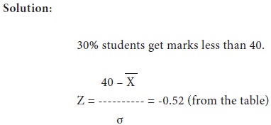
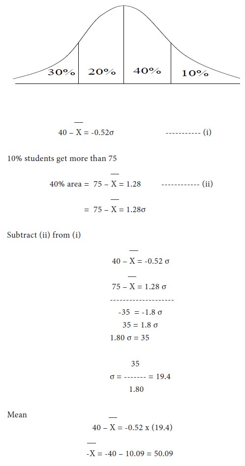
Illustration:
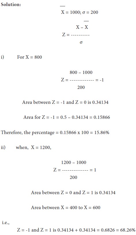
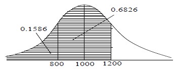
The scores observed by candidate in a certain test are normally distributed with mean 1000 and standard deviation 200. What per cent of candidates receive scores (i) less than 800, (ii) between 800 and 1200? (the area under the curve between Z = 0 and Z = 1 is 0.34134).
10. Skewness = 0 and Kurtosis = 3 in normal distribution.
Find the probability that the standard normal value lies between 0 and 1.5
As the mean, Z = 0.
To find the area between Z = 0 and Z = 1.5, look the area between 0 and 1.5, from the table. It is 0.4332 (shaded area)
Illustration:
The results of a particular examination are given below in a summary form:
It is known that a candidate gets plucked if he obtains less than 40 marks, out of 100 while he must obtain at least 75 marks in order to pass with distinction. Determine the mean and standard deviation of the distribution of marks assuming this to be normal.
Illustration:
The scores observed by candidate in a certain test are normally distributed with mean 1000 and standard deviation 200. What per cent of candidates receive scores (i) less than 800, (ii) between 800 and 1200? (the area under the curve between Z = 0 and Z = 1 is 0.34134).
Tags : Research Methodology - Statistical Analysis
Last 30 days 2135 views