


Research Methodology - Statistical Analysis
CHI-SQUARE TEST - Statistical Analysis
Posted On :
F, t and Z tests are based on the assumption that the samples were drawn from normally distributed populations.
CHI-SQUARE TEST
F, t and Z tests are based on the assumption that the samples were drawn from normally distributed populations. The testing procedure requires assumption about the type of population or parameters, and these tests are known as ‘parametric tests’.
There are many situations in which it is not possible to make any rigid assumption about the distribution of the population from which samples are being drawn. This limitation has led to the development of a group of alternative techniques known as non-parametric tests. Chi-square test of independence and goodness of fit is a prominent example of the use of non-parametric tests.
Though non-parametric theory developed as early as the middle of the nineteenth century, it was only after 1945 that non-parametric tests came to be used widely in sociological and psychological research. The main reasons for the increasing use of non-parametric tests in business research are:-
1. These statistical tests are distribution-free
2. They are usually computationally easier to handle and understand than parametric tests; and
3. They can be used with type of measurements that prohibit the use of parametric tests.
The χ2 test is one of the simplest and most widely used non-parametric tests in statistical work. It is defined as:
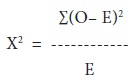
Where
O = the observed frequencies, and E = the expected frequencies.
Steps:
The steps required to determine the value of χ2 are:
Where
E = Expected frequency, R = row’s total of the respective cell, C = column’s total of the respective cell and N = the total number of observations.
The computed value of χ2 is compared with the table value of χ2 for given degrees of freedom at a certain specified level of significance. If at the stated level, the calculated value of χ2 is less than the table value, the difference between theory and observation is not considered as significant.
The following observation may be made with regard to the χ2 distribution:-
F, t and Z tests are based on the assumption that the samples were drawn from normally distributed populations. The testing procedure requires assumption about the type of population or parameters, and these tests are known as ‘parametric tests’.
There are many situations in which it is not possible to make any rigid assumption about the distribution of the population from which samples are being drawn. This limitation has led to the development of a group of alternative techniques known as non-parametric tests. Chi-square test of independence and goodness of fit is a prominent example of the use of non-parametric tests.
Though non-parametric theory developed as early as the middle of the nineteenth century, it was only after 1945 that non-parametric tests came to be used widely in sociological and psychological research. The main reasons for the increasing use of non-parametric tests in business research are:-
1. These statistical tests are distribution-free
2. They are usually computationally easier to handle and understand than parametric tests; and
3. They can be used with type of measurements that prohibit the use of parametric tests.
The χ2 test is one of the simplest and most widely used non-parametric tests in statistical work. It is defined as:
Where
O = the observed frequencies, and E = the expected frequencies.
Steps:
The steps required to determine the value of χ2 are:
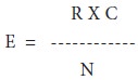
(i) Calculate the expected
frequencies. In general the expected frequency for any cell can be calculated
from the following equation:
Where
E = Expected frequency, R = row’s total of the respective cell, C = column’s total of the respective cell and N = the total number of observations.
(ii) Take the difference between
observed and expected frequencies and obtain the squares of these differences.
Symbolically, it can be represented as (O – E)2
(iii) Divide the values of (O – E)2 obtained in step (ii) by the
respective expected frequency and obtain the total, which can be symbolically
represented by ∑[(O – E)2/E]. This
gives the value of χ2 which
can range from zero to infinity. If χ2 is zero it means that the observed and expected frequencies completely
coincide. The greater the discrepancy between the observed and expected
frequencies, the greater shall be the value of χ2.
The computed value of χ2 is compared with the table value of χ2 for given degrees of freedom at a certain specified level of significance. If at the stated level, the calculated value of χ2 is less than the table value, the difference between theory and observation is not considered as significant.
The following observation may be made with regard to the χ2 distribution:-
i. The sum of the
observed and expected frequencies is always zero. Symbolically, ∑(O – E) = ∑O - ∑E = N – N =
0
ii. The χ2 test depends only on the set of
observed and expected frequencies and on degrees of freedom v. It is a
non-parametric test.
iii. χ2 distribution is a limiting approximation of the multinomial
distribution.
iv. Even though χ2 distribution is essentially a continuous distribution it can be applied to discrete random variables whose frequencies can be counted and tabulated with or without grouping.
iv. Even though χ2 distribution is essentially a continuous distribution it can be applied to discrete random variables whose frequencies can be counted and tabulated with or without grouping.
Tags : Research Methodology - Statistical Analysis
Last 30 days 889 views