


Research Methodology - Statistical Analysis
BINOMIAL DISTRIBUTION - Statistical Analysis
Posted On :
The binomial distribution also known as ‘Bernoulli Distribution’ is associated with the name of a Swiss mathematician, James Bernoulli who is also known as Jacques or Jakon (1654 – 1705).
BINOMIAL DISTRIBUTION
The binomial distribution also known as ‘Bernoulli Distribution’ is associated with the name of a Swiss mathematician, James Bernoulli who is also known as Jacques or Jakon (1654 – 1705). Binomial distribution is a probability distribution expressing the probability of one set of dichotomous alternatives. It can be explained as follows:
1. If an experiment is repeated under the same conditions for a fixed number of trials, say, n.
2. In each trial, there are only two possible outcomes of the experiment. Let us define it as “success” or “failure”. Then the sample space of possible outcomes of each experiment is:
3. S = [failure, success]
4. The probability of a success denoted by p remains constant from trial to trial and the probability of a failure denoted by q which is equal to (1 – p).
5. The trials are independent in nature i.e., the outcomes of any trial or sequence of trials do not affect the outcomes of subsequent trials. Hence, the multiplication theorem of probability can be applied for the occurrence of success and failure. Thus, the probability of success or failure is p.q.
6. Let us assume that we conduct an experiment in n times. Out of which x times be the success and failure is (n-x) times. The occurrence of success or failure in successive trials is mutually exclusive events. Hence, we can apply addition theorem of probability.
7. Based on the above two theorems, the probability of success or failure is

where p = probability of success in a single trail, q = 1 – p, n = Number of trials and x = no. of successes in n trials.
Thus, for an event A with probability of occurrence p and non-occurrence q, if n trials are made, probability distribution of the number of occurrences of A will be as set. If we want to obtain the probable frequencies of the various outcomes in n sets of N trials, the following expression shall be used: N(p + q)n

The frequencies obtained by the above expansion are known as expected or theoretical frequencies. On the other hand, the frequencies actually obtained by making experiments are called actual or observed frequencies. Generally, there is some difference between the observed and expected frequencies but the difference becomes smaller and smaller as N increases.
The following rules may be considered for obtaining coefficients from the binomial expansion:
1. The first term is qn.,
2. The second term is nC1qn-1p,
3. In each succeeding term the power of q is reduced by 1 and the power of p is increased by 1.
4. The coefficient of any term is found by multiplying the coefficient of the preceding term by the power of q in that preceding term, and dividing the products so obtained by one more than the power of p in that proceeding term.
Thus, when we expand (q + p)n,
we will obtain the following:-

Where, 1, nC1, nC2 ……. are called the binomial coefficient. Thus in the expansion of (p + q)4 we will have (p + q)4 = p4 +4p3q +6p2q2 + 4p1q3 + q4 and the coefficients will be 1, 4, 6, 4, 1.
From the above binomial expansion, the following general relationships should be noted:
1. The number of terms in a binomial expansion is always n + 1,
2. The exponents of p and q, for any single term, when added together, always sum to n.
3. The exponents of p are n, (n – 1), (n – 2),…….1, 0, respectively and the exponents of q are 0, 1, 2, ……(n – 1), n, respectively.
4. The coefficients for the n + 1 terms of the distribution are always symmetrical in nature.
The main properties of binomial distribution are:-
1. The shape and location of binomial distribution changes as p changes for a given n or as n changes for a given p. As p increases for a fixed n, the binomial distribution shifts to the right.
2. The mode of the binomial distribution is equal to the value of x which has the largest probability. The mean and mode are equal if np is an integer.
3. As n increases for a fixed p, the binomial distribution moves to the right, flattens and spreads out.
4. The mean of the binomial distribution is np and it increases as n increases with p held constant. For larger n there are more possible outcomes of a binomial experiment and the probability associated with any particular outcome becomes smaller.
Illustrations:
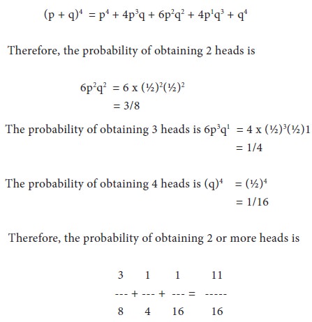
A coin is tossed four times. What is the probability of obtaining two or more heads?
Solution:
when a coin is tossed the probabilities of head and tail in case of an unbiased coin are equal, i.e., p = q = ½
The various possibilities for all the events are the terms of the expansion (q+p)4
The binomial distribution also known as ‘Bernoulli Distribution’ is associated with the name of a Swiss mathematician, James Bernoulli who is also known as Jacques or Jakon (1654 – 1705). Binomial distribution is a probability distribution expressing the probability of one set of dichotomous alternatives. It can be explained as follows:
1. If an experiment is repeated under the same conditions for a fixed number of trials, say, n.
2. In each trial, there are only two possible outcomes of the experiment. Let us define it as “success” or “failure”. Then the sample space of possible outcomes of each experiment is:
3. S = [failure, success]
4. The probability of a success denoted by p remains constant from trial to trial and the probability of a failure denoted by q which is equal to (1 – p).
5. The trials are independent in nature i.e., the outcomes of any trial or sequence of trials do not affect the outcomes of subsequent trials. Hence, the multiplication theorem of probability can be applied for the occurrence of success and failure. Thus, the probability of success or failure is p.q.
6. Let us assume that we conduct an experiment in n times. Out of which x times be the success and failure is (n-x) times. The occurrence of success or failure in successive trials is mutually exclusive events. Hence, we can apply addition theorem of probability.
7. Based on the above two theorems, the probability of success or failure is
where p = probability of success in a single trail, q = 1 – p, n = Number of trials and x = no. of successes in n trials.
Thus, for an event A with probability of occurrence p and non-occurrence q, if n trials are made, probability distribution of the number of occurrences of A will be as set. If we want to obtain the probable frequencies of the various outcomes in n sets of N trials, the following expression shall be used: N(p + q)n
The frequencies obtained by the above expansion are known as expected or theoretical frequencies. On the other hand, the frequencies actually obtained by making experiments are called actual or observed frequencies. Generally, there is some difference between the observed and expected frequencies but the difference becomes smaller and smaller as N increases.
Obtaining Coefficient Of The Binomial Distribution:
The following rules may be considered for obtaining coefficients from the binomial expansion:
1. The first term is qn.,
2. The second term is nC1qn-1p,
3. In each succeeding term the power of q is reduced by 1 and the power of p is increased by 1.
4. The coefficient of any term is found by multiplying the coefficient of the preceding term by the power of q in that preceding term, and dividing the products so obtained by one more than the power of p in that proceeding term.
Where, 1, nC1, nC2 ……. are called the binomial coefficient. Thus in the expansion of (p + q)4 we will have (p + q)4 = p4 +4p3q +6p2q2 + 4p1q3 + q4 and the coefficients will be 1, 4, 6, 4, 1.
From the above binomial expansion, the following general relationships should be noted:
1. The number of terms in a binomial expansion is always n + 1,
2. The exponents of p and q, for any single term, when added together, always sum to n.
3. The exponents of p are n, (n – 1), (n – 2),…….1, 0, respectively and the exponents of q are 0, 1, 2, ……(n – 1), n, respectively.
4. The coefficients for the n + 1 terms of the distribution are always symmetrical in nature.
Properties Of Binomial Distribution
The main properties of binomial distribution are:-
1. The shape and location of binomial distribution changes as p changes for a given n or as n changes for a given p. As p increases for a fixed n, the binomial distribution shifts to the right.
2. The mode of the binomial distribution is equal to the value of x which has the largest probability. The mean and mode are equal if np is an integer.
3. As n increases for a fixed p, the binomial distribution moves to the right, flattens and spreads out.
4. The mean of the binomial distribution is np and it increases as n increases with p held constant. For larger n there are more possible outcomes of a binomial experiment and the probability associated with any particular outcome becomes smaller.
5. If n is larger and if neither p
nor q is too close to zero, the binomial distribution can be closely
approximated by a normal distribution with standardized variable given by z =
(X – np) / √npq.
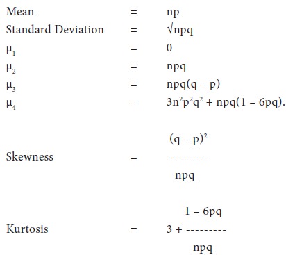
6. The various constants of binomial distribution are:
6. The various constants of binomial distribution are:
Illustrations:
A coin is tossed four times. What is the probability of obtaining two or more heads?
Solution:
when a coin is tossed the probabilities of head and tail in case of an unbiased coin are equal, i.e., p = q = ½
The various possibilities for all the events are the terms of the expansion (q+p)4
Illustration:
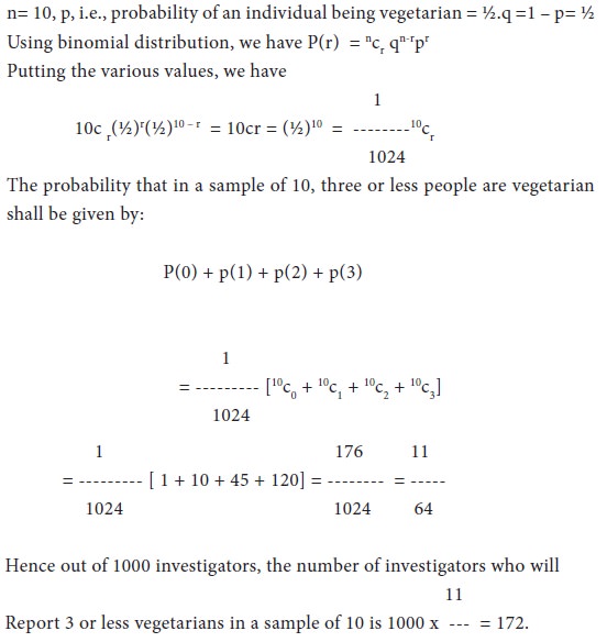
Assuming that half the population is vegetarian so that the chance of an individual being a vegetarian is ½ and assuming that 100 investigations can take sample of 10 individuals to verify whether they are vegetarians, how many investigation would you expect to report that three people or less were vegetarians?
Solution:
Tags : Research Methodology - Statistical Analysis
Last 30 days 861 views