Big-M Method [Introduction]

In order to obtain an initial basic feasible solution, it is necessary to convert the given LPP into its standard form; in order to obtain the standard form; a non-negative variable is added to the left side of each of the equation that lacks the much needed starting basic variables. So added variable is called an artificial variable and it places the role in providing initial basic feasible solution.

Big-M Method [Introduction]

 

In order to obtain an initial basic feasible solution, it is necessary to convert the given LPP into its standard form; in order to obtain the standard form; a non-negative variable is added to the left side of each of the equation that lacks the much needed starting basic variables. So added variable is called an artificial variable and it places the role in providing initial basic feasible solution.

 

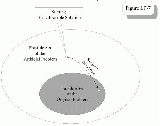
The starting point of the big-M method is a basic solution that is feasible to the artificial problem. This solution allows us to start the Simplex algorithm expeditiously, but it is not a feasible solution to the original problem. Our goal is to iterate toward solutions that are inside the original feasible set, assuming that it is not empty.

 

The artificial variables have no physical meaning from the view of the original problem; the method will be valid only if it is possible to force these variables at zero level when the optimum solution is attained.

To accomplish this goal, we designed an artificial objective function that is an aggregation of two functional parts, of which one is a copy of the original objective function and the other is a “penalty function” associated with the artificial variables.

 

The magnitude of the penalty, M, needs to be chosen to ensure that the contribution to this aggregate objective function from the second part, whenever it is positive, always outweighs that from the first part, for any solution.

 

Artificial Variable

 

 

If there is a constraint which is of > = or equality type then it is needed to write the constraint in standard form because it is not possible to get unit column vector. The additional variable, which is added in order to get unit column vector, is called an artificial variable.

 

Two methods are generally employed for the solution of linear programming problems having artificial variables:

 

1.  Two-Phase Method.

 

2.  Big-M Method (or) Method of Penalties. We will have discussion only on Big-M Method here.

 

The Big M Method Procedure

 

 

If an LP has any > or = constraints, the Big M method or the two-phase simplex method may be used to solve the problem.

 

The Big M method is a version of the Simplex Algorithm that first finds a best feasible solution by adding “artificial” variables to the problem. The objective function of the original LP must, of course, be modified to ensure that the artificial variables are all equal to 0 at the conclusion of the simplex algorithm. The iterative procedure of the algorithm is given below.

 

Step-1

 

 

Modify the constraints so that the RHS of each constraint is non-negative (This requires that each constraint with a negative RHS be multiplied by -1. Remember that if any negative number multiplies an inequality, the direction of the inequality is reversed). After modification, identify each constraint as a <, >, or = constraint.

 

Step-2

 

 

Convert each inequality constraint to standard form (If a constraint is a ≤ constraint, then add a slack variable Xi; and if any constraint is a ≥ constraint, then subtract an excess variable Xi , known as surplus variable).

 

Step-3

 

 

Add an artificial variable a1 to the constraints identified as ‘≥’ or with ‘=’ constraints at the end of Step2. Also add the sign restriction ai ≥ 0.

 

 

Step-4

 

 

Let M denote a very large positive number. If the LP is a minimization problem, add (for each artificial variable) Mai to the objective function. If the LP is a maximization problem, add (for each artificial variable) -Mai to the objective function.

 

Step-5

 

 

Since each artificial variable will be in the starting basis, all artificial variables must be eliminated from row 0 before beginning the simplex.

 

Now we solve the transformed problem by the simplex (In choosing the entering variable, remember that M is a very large positive number). If all artificial variables are equal to zero in the optimal solution, we have found the optimal solution to the original problem. If any artificial variables are positive in the optimal solution, the original problem is infeasible!!!

 

1. If at least one artificial variable is present in the basis with zero value, in such a case the current optimum basic feasible solution is a degenerate solution.

 

2. If at least one artificial variable is present in the basis with a positive value, then in such a case, the given LPP does not have an optimum basic feasible solution. The given problem is said to have a pseudo-optimum basic feasible solution.

 

Example-1

 

 

Solve the following LPP by using Big -M Method

 

Maximize Z = 6X1+4X2

 

Subject to constraints:

 

2X1+3X2<=30

 

3X1+2X2<=24

 

X1+X2>=3

 

 

Solution

 

 

Introducing slack variables S1>=0, S2>=0 to the first and second equations in order to convert <= type to equality and add surplus variable to the third equation S3 >=0 to convert >= type to equality.

 

Then the standard form of LPP is

 

MAX Z=6X1+4X2+0S1+0S2+0S3 Subject to constraints

 

2X1+3X2+S1=30

 

3X1+2X2+S2=24

 

X1+X2-S3=3

 

Clearly there is no initial basic feasible solution. So an artificial variable A1>=0 is added in the third equation. Now the standard form will be

 

MAX Z=6X1+4X2+0S1+0S2+0S3+A1

 

Subject to constraints

 

2X1+3X2+S1=30

 

3X1+2X2+S2=24

 

X1+X2-S3+A1=3

 

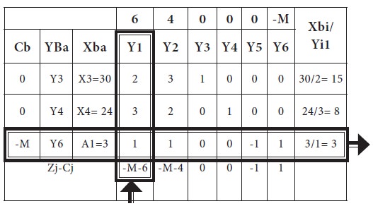
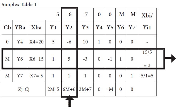
Now the first simplex table is placed below with following additional information.

 

It clearly shows the net evaluations for each column variable; from these calculations, it is clear that X1 is the entering variable and A1, the artificial variable leaves the basis. Introduce Y1 and drop Y6

Then, in the usual row operations, we modify this table and the new table is arrived.

 

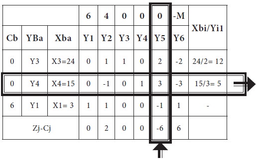
Table-2

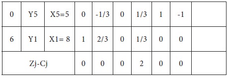
Introduce Y5 and drop Y4 from the basis; the new modified table-3 is given below;

Since all Zj –Cj >=0, an optimum solution has reached. Thus an optimum basic feasible solution to the LPP is

 

X1=8

 

X2=0

 

MAX Z =48

 

 

Example-2

 

 

Use big M method to solve a given LPP. Minimize Z = 5X1-6X2-7X3

 

Subject to constraints

 

X1+5X2-3X3>=15

 

5X1-6X2+10X3<=20

 

X1+X2+X3=5

 

X1, X2 & X3 >= 0

 

Solution

 

 

Introducing slack variables X4>=0 to the first equations in order to convert <= type to equality and add surplus variable X5>=0 to the second equation in order to convert >= type to equality.

 

Then the standard form of LPP is

 

MIN Z=5X1-6X2-7X3+X4-X5 Subject to constraints

 

5X1-6X2+10X3+X4=20

 

X1+5X2-3X3-X5=15

 

X1+X2+X3=5

 

Clearly there is no initial basic feasible solution. So two artificial variables A1>=0 and A2>=0 are added in the second and third equation. Now the standard form will be

 

MIN Z=5X1-6X2-7X3+X4-X5+A1+A2 Subject to constraints

 

5X1-6X2+10X3+X4=20

 

X1+5X2-3X3-X5+A1=15

 

X1+X2+X3+A2=5

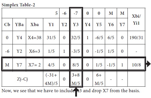
From the calculations related to entering column and leaving variable, which is summarized in the above table, it is clear that introduces X2 and drop X6 from the basis. The new simplex table is given below;

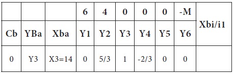
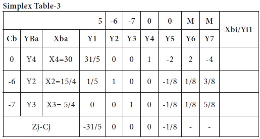
The new modified table- 3 is given below

 

-1/5 +32/5*1/5*5/8

Since all Zj –Cj <=0, an optimum solution has reached. Thus an optimum basic feasible solution to the LPP is

 

X3=5/4

 

X2=15/4

 

MIN Z= (5*0) + (-6*15/4) + (-7* 5/4)

 

=   (-90/4) + (-35/4)

 

=   -125/4