


Home | ARTS | Operations Management
|
GRAPHICAL SOLUTION PROCEDURE OF LP PROBLEMS - Linear Programming – Problem Solving [GRAPHICAL METHOD]
Operations Management - Introduction to Operations Research
GRAPHICAL SOLUTION PROCEDURE OF LP PROBLEMS - Linear Programming – Problem Solving [GRAPHICAL METHOD]
Posted On :
While obtaining the optimal solution to the LP problem by the graphical method, the statement of the following theorems of linear programming is used.
GRAPHICAL SOLUTION PROCEDURE OF
LP PROBLEMS
While obtaining the optimal solution to the LP problem by the graphical method, the statement of the following theorems of linear programming is used.
1. The collection of all feasible solutions to an LP problem constitutes a convex set whose extreme points correspond to the basic feasible solutions.
2. There are a finite number of basic feasible solutions within the feasible solution space.
3. If the convex set of the feasible solutions of the system Ax=b, x>=0, is a convex polyhedron, then at least one of the extreme points gives an optimal solution.
4. If the optimal solution occurs at more than one extreme point, then the value of the objective function will be the same for all convex combinations of these extreme points.
This solution method for an LP problem is divided into five steps.
State the given problem in the mathematical form.
Graph the constraints, by temporarily ignoring the inequality sign and decide about the area of feasible solutions according to the inequality sign of the constraints. Indicate
Determine the coordinates of the extreme points of the feasible solution space.
Evaluate the value of the objective function at each extreme point.
Determine the extreme point to obtain the optimum (best) value of the objective function.
Example-1
Use the graphical method to solve the following LPP problem:
Maximize z = 15X1 + 10X2
Subject to constraints
4X1+6X2 <=360
3X1+0X2<=180
0X1+5X2 <=200
X1, X2>=0
Solution
Step 1
State the problem in mathematical form.
The problem we have considered here is already in mathematical form [given in terms of mathematical symbols and notations]
Step 2
Plot the constraints on the graph paper and find the feasible region.
We shall treat x1 as the horizontal axis and x2 as the vertical axis. Each constraint will be plotted on the graph by treating it as a linear equation and then appropriate inequality conditions will be used to mark the area of the feasible solutions.
Consider the first constraint 4X1+6X2<=360 .Treated it as the equation,
4X1+6X2 =360.
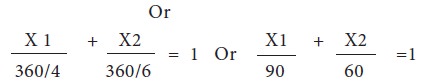
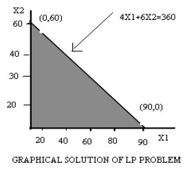
This equation indicates that when it is plotted, the graph cuts X1 axis [intercept] at 90 and X2 axis [x2 intercept] at 60. These two points are then connected by a straight line as shown in figure.
But the inequality and non-negativity condition can only be satisfied by the shaded area (feasible region) as shown in figure below:
Similarly the constraints 3X1<=180 and 5X2<=200 are also plotted on the same graph, which is shown above and the required region is indicated by the shaded area, which is common to all the 3 constraint as shown in figure below:
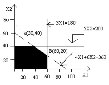
Since all constraints have been graphed, the area which is bounded by all the constraints lines including all the boundary points is called the feasible region or solution space. The feasible region is shown in fig by the area OABCD.
Step 3
Determine the coordinates of extreme points
Since the optimal value of the objective function occurs at one of the extreme points of the feasible region, it is necessary to determine their coordinates. The coordinates of extreme points of the feasible region are:
O = (0, 0),
A= (60, 0)
B= (60, 20),
C= (30, 40),
D= (0, 40)
Step 4
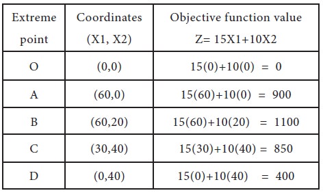
Evaluate the value of the objective at extreme points Now, the next step is to evaluate the objective function value at each extreme point of the feasible region, which is shown below:
Step 5
Determining the optimal value of the objective function Since our desire it to maximize the value of the objective function, Z, therefore from step 4 we can conclude that maximum value of Z=1100 is achieved at the point B (60, 20). Hence the optimal solution to the given LP problem is:
X1=60,
X2=20 and
Value of the objective function, Z=1100
Example-2: Use the graphical method to solve the following LP problem
Minimize Z=20X1+10X2
Subject to constraints,
X1+2X2 ≤
40
3X1+X2 ≥ 30
4X1+3X2 ≥ 60
And X1, X2 ≥ 0
Solution
Step 1
State the problem in mathematical form.
The problem we have considered here is already in mathematical form [given in terms of mathematical symbols and notations]
Step 2
Plot the constraints on the graph paper and find the feasible region.
We shall treat x1 as the horizontal axis and x2 as the vertical axis. Each constraint will be plotted on the graph by treating it as a linear equation and then appropriate inequality conditions will be used to mark the area of the feasible solutions.
The constraints are written in the following form;
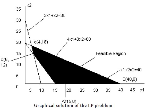
Graph each constraint by first treating it as a linear equation. Then use the inequality condition of each constraint to make the feasible region as shown in following figure.
Step 3
Determine the coordinates of extreme points
Since the optimal value of the objective function occurs at one of the extreme points of the feasible region, it is necessary to determine their coordinates. The coordinates of extreme points of the feasible region are:
A= (15, 0), B= (40, 0),C= (4, 18) and D= (6, 12).
Step 4
Evaluate the value of the objective at extreme points Now, the next step is to evaluate the objective function value at each extreme point of the feasible region, which is shown below:
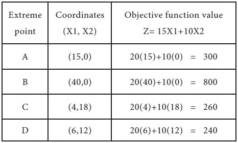
Therefore, the minimum value of the objective function Z=240 occurs at the extreme point D (6, 12).
Hence, the optimal solution to the given LP problem is:
X1 = 6, X2 = 12
And the value of the objective function is
Z = 240.
While obtaining the optimal solution to the LP problem by the graphical method, the statement of the following theorems of linear programming is used.
1. The collection of all feasible solutions to an LP problem constitutes a convex set whose extreme points correspond to the basic feasible solutions.
2. There are a finite number of basic feasible solutions within the feasible solution space.
3. If the convex set of the feasible solutions of the system Ax=b, x>=0, is a convex polyhedron, then at least one of the extreme points gives an optimal solution.
4. If the optimal solution occurs at more than one extreme point, then the value of the objective function will be the same for all convex combinations of these extreme points.
METHOD-1: Extreme Point Enumeration Approach
This solution method for an LP problem is divided into five steps.
Step 1
State the given problem in the mathematical form.
Step 2
Graph the constraints, by temporarily ignoring the inequality sign and decide about the area of feasible solutions according to the inequality sign of the constraints. Indicate
Step 3
Determine the coordinates of the extreme points of the feasible solution space.
Step 4
Evaluate the value of the objective function at each extreme point.
Step 5
Determine the extreme point to obtain the optimum (best) value of the objective function.
Example-1
Use the graphical method to solve the following LPP problem:
Maximize z = 15X1 + 10X2
Subject to constraints
4X1+6X2 <=360
3X1+0X2<=180
0X1+5X2 <=200
X1, X2>=0
Solution
Step 1
State the problem in mathematical form.
The problem we have considered here is already in mathematical form [given in terms of mathematical symbols and notations]
Plot the constraints on the graph paper and find the feasible region.
We shall treat x1 as the horizontal axis and x2 as the vertical axis. Each constraint will be plotted on the graph by treating it as a linear equation and then appropriate inequality conditions will be used to mark the area of the feasible solutions.
Consider the first constraint 4X1+6X2<=360 .Treated it as the equation,
This equation indicates that when it is plotted, the graph cuts X1 axis [intercept] at 90 and X2 axis [x2 intercept] at 60. These two points are then connected by a straight line as shown in figure.
But the inequality and non-negativity condition can only be satisfied by the shaded area (feasible region) as shown in figure below:
Similarly the constraints 3X1<=180 and 5X2<=200 are also plotted on the same graph, which is shown above and the required region is indicated by the shaded area, which is common to all the 3 constraint as shown in figure below:
Since all constraints have been graphed, the area which is bounded by all the constraints lines including all the boundary points is called the feasible region or solution space. The feasible region is shown in fig by the area OABCD.
Step 3
Determine the coordinates of extreme points
Since the optimal value of the objective function occurs at one of the extreme points of the feasible region, it is necessary to determine their coordinates. The coordinates of extreme points of the feasible region are:
O = (0, 0),
A= (60, 0)
B= (60, 20),
C= (30, 40),
D= (0, 40)
Step 4
Evaluate the value of the objective at extreme points Now, the next step is to evaluate the objective function value at each extreme point of the feasible region, which is shown below:
Step 5
Determining the optimal value of the objective function Since our desire it to maximize the value of the objective function, Z, therefore from step 4 we can conclude that maximum value of Z=1100 is achieved at the point B (60, 20). Hence the optimal solution to the given LP problem is:
X1=60,
X2=20 and
Value of the objective function, Z=1100
Example-2: Use the graphical method to solve the following LP problem
Minimize Z=20X1+10X2
Subject to constraints,
3X1+X2 ≥ 30
4X1+3X2 ≥ 60
And X1, X2 ≥ 0
Solution
Step 1
State the problem in mathematical form.
The problem we have considered here is already in mathematical form [given in terms of mathematical symbols and notations]
Step 2
Plot the constraints on the graph paper and find the feasible region.
We shall treat x1 as the horizontal axis and x2 as the vertical axis. Each constraint will be plotted on the graph by treating it as a linear equation and then appropriate inequality conditions will be used to mark the area of the feasible solutions.
The constraints are written in the following form;
X1/40 + X2/(40/2) ≤ 1 or | X1/40 +
X2/20 ≤ 1----- | (1) |
X1/(30/3) + X2/3 ≥ 1 or | X1/10 +
X2/30 ≤ 1---- | (2) |
X1/(60/4) + X2/(60/3) ≥ 1 or X1/15 + X2/20 ≥
1-------------- | (3) | |
Graph each constraint by first treating it as a linear equation. Then use the inequality condition of each constraint to make the feasible region as shown in following figure.
Step 3
Determine the coordinates of extreme points
Since the optimal value of the objective function occurs at one of the extreme points of the feasible region, it is necessary to determine their coordinates. The coordinates of extreme points of the feasible region are:
A= (15, 0), B= (40, 0),C= (4, 18) and D= (6, 12).
Step 4
Evaluate the value of the objective at extreme points Now, the next step is to evaluate the objective function value at each extreme point of the feasible region, which is shown below:
Therefore, the minimum value of the objective function Z=240 occurs at the extreme point D (6, 12).
Hence, the optimal solution to the given LP problem is:
X1 = 6, X2 = 12
And the value of the objective function is
Z = 240.
Tags : Operations Management - Introduction to Operations Research
Last 30 days 4815 views