


Home | ARTS | Operations Management
|
Some Special Cases of Graphical Solution Methods of Lp Problems - Linear Programming – Problem Solving [GRAPHICAL METHOD]
Operations Management - Introduction to Operations Research
Some Special Cases of Graphical Solution Methods of Lp Problems - Linear Programming – Problem Solving [GRAPHICAL METHOD]
Posted On :
Some Special Cases of Graphical Solution Methods of Lp Problems
Some Special Cases of Graphical Solution Methods of
Lp Problems
Case-1: No Feasible Solution space
Consider the following LPP
Max Z= 4X1 + 4 X2
Subject to
2X1 + 2X2 >= 12
3X1 + 3X2 <= 9
X1, X2 >= 0
The solution is arrived through the graphical method; various steps are given below.
We plot the first constraint in the graphical plane
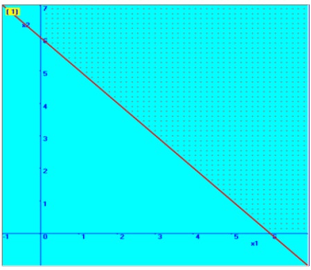
Consider 2X1 + 2X2 = 12
If X1 = 0, then X2 = 6
Therefore, one point on the line is (0, 6)
If X2 =0, then X1 = 6
Therefore another point on the line is (6, 0)
We will fix with the help of these two points in the graphical plane, which is shown here. Then, based on the inequality sign, the required region is marked here.
In similar way, we fixed the second constraint
3X1 + 3X2 = 9
If X1 = 0, then X2 = 3
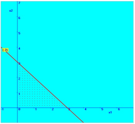
Therefore, one point on the line is (0, 3)
If X2 =0, then X1 = 3
Therefore another point on the line is (3, 0)
We will fix straight line with the help of these two points in the graphical plane, which is shown here. Then, based on the inequality sign, the required region is marked here.
Then the combined graphical solution space is arrived and shown here in the diagram.
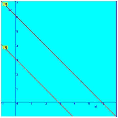
You can note that there is no common solution area between these two constraints.
Hence this kind of problem is categorized as ‘No Feasible solution’.
Case-2: Unbounded Solution space
Consider the following LPP
Max Z= 4X1 + 4 X2
Subject to
2X1 + 2X2 >= 12
3X2 <= 9
X1, X2 >= 0
The solution is arrived through the graphical method; various steps are given below.
We plot the first constraint in the graphical plane
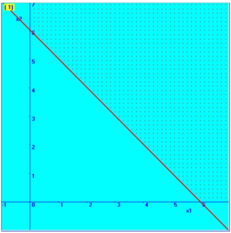
Consider 2X1 + 2X2 = 12
If X1 = 0, then X2 = 6
Therefore, one point on the line is (0, 6)
If X2 =0, then X1 = 6
Therefore another point on the line is (6, 0)
We will fix with the help of these two points in the graphical plane, which is shown here. Then, based on the inequality sign, the required region is marked here.
In similar way, we fixed the second constraint;
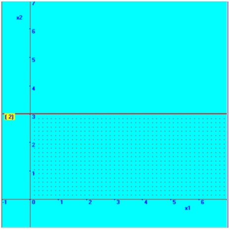
Therefore, the straight line is parallel to X1 axis and passes through X2=3
Now, we fixed the straight line with the help of this point in the graphical plane, which is shown here. Then, based on the inequality sign, the required region is marked here.
Then the combined graphical solution space is arrived and shown below in the diagram.
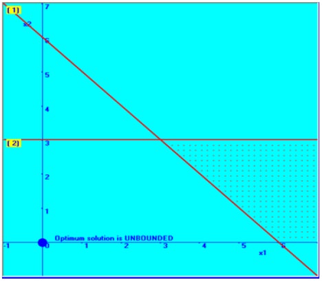
You can note that the solution area between these
two constraints is not bounded one; that is there is no finite solution space
and this has implied that the solution can be infinitely increased with the
limited resources. This is not obviously possible. Hence this kind of problem
is categorized as ‘unbounded feasible solution’.
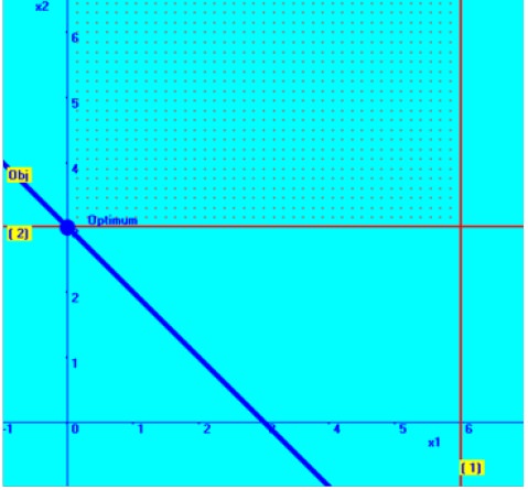
Case-3: Unbounded Solution space-possibility of optimum solution Consider the following LPP
Min Z= 4X1 + 4 X2
Subject to
2X1 + 0X2<= 12
0X1+ 3X2 <= 9
X1, X2 >= 0
The solution is arrived through the graphical method; various steps are given below.
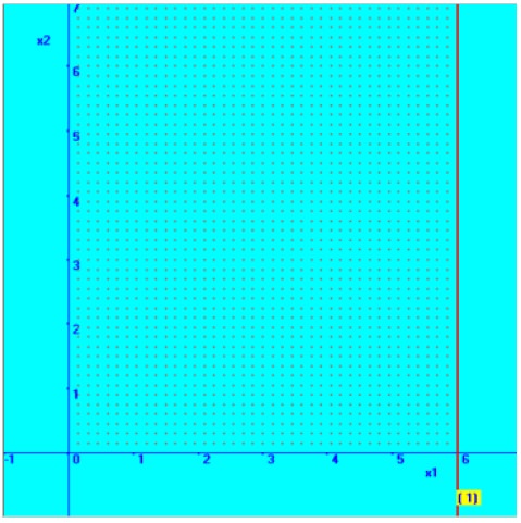
Consider the first constraint-2X1 + <= 12
From this constraint, we consider the following straight line equation,
Therefore, the straight line is parallel to X2 axis and passes through X1=6
Then the required region for the constraint, 2X1 + <= 12 is deducted by substituting an arbitrary point – say origin (0, 0) and check whether it is satisfied by the constraint. It is shown below in the diagram.
Then the required region for the constraint, 3X2 <= 9 is deducted by substituting an arbitrary point – say origin (0, 0) and check whether it is satisfied by the constraint. It is shown above in the diagram.
In the diagram in the right hand side, the combined graphical solution space is shown.
You can
notice that there exists an optimum solution, even though the solution space is
not bounded.
At X1=0 & X2= 2, there is
minimum value obtained for the problem.
Case-4: Multiple Optimum Solutions -possibility of more than one
optimum solution
Consider the following LPP.
Max Z = X1 + 2X2
Subject to
X1 + 2X2 ≤ 10
X1 + X2 ≥ 1
X2 ≤ 4
X1 & X2 ≥0
Consider the straight line equation,
Therefore, one point on the line is (0, 5)
Therefore another point on the line is (10, 0)
We will
fix with the help of these two points in the graphical plane, which is shown
here. Then, based on the inequality sign, the required region is marked here.
Consider the second constraint,
X1 + X2 ≥ 1
Now the respective straight line equation is considered for fixing the line.
Therefore, one point on the line is (0, 1)
Therefore another point on the line is (1, 0).
We will
fix with the help of these two points in the graphical plane, which is shown
here. To fix the required region, we take arbitrary point, (0, 0) and
substituting the values, in the second constraint, we find that it is not
satisfying the inequality. Therefore, the region, above the straight line forms
the required region.
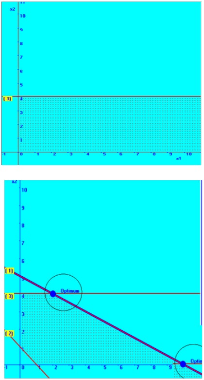
In a similar way, the third constraint is also
placed in the graphical plane and the combined picture of all the straight
lines is also placed below with the solution space.
You can notice that the present problem, at two points, there is a possibility of getting maximum value for the objective function.
At X1= 2 & X2 = 4, the objective function value, Z = 10 And X1 = 10 & X2=0, again the objective function value,
Z = 10
These kinds of problems are called as linear programming problem with multiple optimum solutions.
Case-1: No Feasible Solution space
Consider the following LPP
Max Z= 4X1 + 4 X2
Subject to
2X1 + 2X2 >= 12
3X1 + 3X2 <= 9
X1, X2 >= 0
The solution is arrived through the graphical method; various steps are given below.
We plot the first constraint in the graphical plane
Consider 2X1 + 2X2 = 12
If X1 = 0, then X2 = 6
Therefore, one point on the line is (0, 6)
If X2 =0, then X1 = 6
Therefore another point on the line is (6, 0)
We will fix with the help of these two points in the graphical plane, which is shown here. Then, based on the inequality sign, the required region is marked here.
In similar way, we fixed the second constraint
3X1 + 3X2 = 9
If X1 = 0, then X2 = 3
Therefore, one point on the line is (0, 3)
If X2 =0, then X1 = 3
Therefore another point on the line is (3, 0)
We will fix straight line with the help of these two points in the graphical plane, which is shown here. Then, based on the inequality sign, the required region is marked here.
Then the combined graphical solution space is arrived and shown here in the diagram.
You can note that there is no common solution area between these two constraints.
Hence this kind of problem is categorized as ‘No Feasible solution’.
Case-2: Unbounded Solution space
Consider the following LPP
Max Z= 4X1 + 4 X2
Subject to
2X1 + 2X2 >= 12
3X2 <= 9
X1, X2 >= 0
The solution is arrived through the graphical method; various steps are given below.
We plot the first constraint in the graphical plane
Consider 2X1 + 2X2 = 12
If X1 = 0, then X2 = 6
Therefore, one point on the line is (0, 6)
If X2 =0, then X1 = 6
Therefore another point on the line is (6, 0)
We will fix with the help of these two points in the graphical plane, which is shown here. Then, based on the inequality sign, the required region is marked here.
In similar way, we fixed the second constraint;
3X2 | = 9 | |
Since, | X1 = 0, | |
then | X2 | = 3 |
Therefore, the straight line is parallel to X1 axis and passes through X2=3
Now, we fixed the straight line with the help of this point in the graphical plane, which is shown here. Then, based on the inequality sign, the required region is marked here.
Then the combined graphical solution space is arrived and shown below in the diagram.
Case-3: Unbounded Solution space-possibility of optimum solution Consider the following LPP
Min Z= 4X1 + 4 X2
Subject to
2X1 + 0X2<= 12
0X1+ 3X2 <= 9
X1, X2 >= 0
The solution is arrived through the graphical method; various steps are given below.
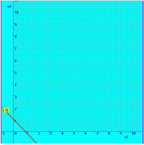
Consider the first constraint-2X1 + <= 12
From this constraint, we consider the following straight line equation,
2X1 = 12 | |
Since, | X2 = 0, |
then | X1 = 6 |
Therefore, the straight line is parallel to X2 axis and passes through X1=6
Then the required region for the constraint, 2X1 + <= 12 is deducted by substituting an arbitrary point – say origin (0, 0) and check whether it is satisfied by the constraint. It is shown below in the diagram.
In a
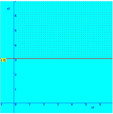
similar way, the second constraint is considered; 0X1+ 3X2 <= 9 From this
constraint, we consider the following straight line equation,
Thus, you can sense that the straight line is parallel to X1 axis and passes through X2=3
3X2 = 9 | ||
Since, | X1 | = 0, |
then | X2 | = 3 |
Thus, you can sense that the straight line is parallel to X1 axis and passes through X2=3
Then the required region for the constraint, 3X2 <= 9 is deducted by substituting an arbitrary point – say origin (0, 0) and check whether it is satisfied by the constraint. It is shown above in the diagram.
In the diagram in the right hand side, the combined graphical solution space is shown.
Case-4: Multiple Optimum Solutions -possibility of more than one
optimum solution
Consider the following LPP.
Max Z = X1 + 2X2
Subject to
X1 + 2X2 ≤ 10
X1 + X2 ≥ 1
X2 ≤ 4
X1 & X2 ≥0
The
solution is arrived through the graphical method; various steps are given
below.
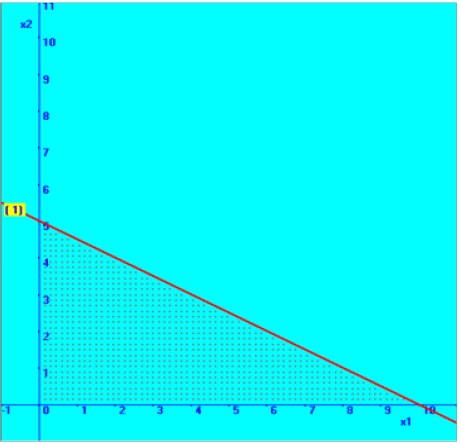
Consider the first constraint X1 + 2X2 ≤ 10
We plot the first constraint in the graphical plane;
Consider the first constraint X1 + 2X2 ≤ 10
We plot the first constraint in the graphical plane;
X1 + 2X2 = 10 | ||
If | X1 | = 0, |
then | X2 | = 5 |
Therefore, one point on the line is (0, 5)
If | X2 | =0, |
then | X1 | = 10 |
Therefore another point on the line is (10, 0)
Now the respective straight line equation is considered for fixing the line.
X1 + X2 = 1 | ||
If | X1 | = 0, |
then | X2 | = 1 |
Therefore, one point on the line is (0, 1)
If | X2 =0, |
then | X1 = 1 |
Therefore another point on the line is (1, 0).
You can notice that the present problem, at two points, there is a possibility of getting maximum value for the objective function.
At X1= 2 & X2 = 4, the objective function value, Z = 10 And X1 = 10 & X2=0, again the objective function value,
Z = 10
These kinds of problems are called as linear programming problem with multiple optimum solutions.
Tags : Operations Management - Introduction to Operations Research
Last 30 days 2118 views