


Home | ARTS | Research Methodology
|
PRINCIPLE OF LEAST SQUARES - Correlation And Regression Analysis
Research Methodology - Correlation And Regression Analysis
PRINCIPLE OF LEAST SQUARES - Correlation And Regression Analysis
Posted On :
Let x, y be two variables under consideration. Out of them, let x be an independent variable and let y be a dependent variable, depending on x. We desire to build a functional relationship between them.
PRINCIPLE OF LEAST SQUARES
Let x, y be two variables under consideration. Out of them, let x be an independent variable and let y be a dependent variable, depending on x. We desire to build a functional relationship between them. For this purpose, the first and foremost requirement is that x, y have a high degree of correlation. If the correlation coefficient between x and y is moderate or less, we shall not go ahead with the task of fitting a functional relationship between them.
Suppose there is a high degree of correlation (positive or negative) between x and y. Suppose it is required to build a linear relationship between them i.e., we want a regression of y on x.
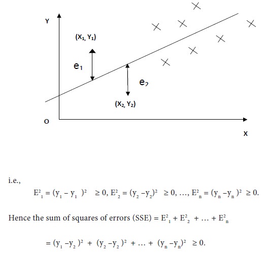
Geometrically speaking, if we plot the corresponding values of x and y in a 2-dimensional plane and join such points, we shall obtain a straight line. However, hardly we can expect all the pairs (x, y) to lie on a straight line. We can consider several straight lines which are, to some extent, near all the points (x, y). Consider one line. An observation (x1, y1) may be either above the line of consideration or below the line. Project this point on the x-axis. It will meet the straight line at the point (x1, y1e). Here the theoretical value (or the expected value) of the variable is y1e while the observed value is y1. When there is a difference between the expected and observed values, there appears an error. This error is E1 = y1 –y1 . This is positive if (x1, y 1) is a point above the line and negative if (x1, y1) is a point below the line. For the n pairs of observations, we have the following n quantities of error:
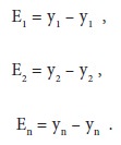
Some of these quantities are positive while the remaining ones are negative. However, the squares of all these quantities are positive.
Among all those straight lines which are somewhat near to the given observations
 we consider that straight line as the ideal one for which the sse is the least. Since the ideal straight line giving regression of y on x is based on this concept, we call this principle as the Principle of least squares.
Suppose we have to fit a straight line to the n pairs of observations Suppose the equation of straight line finally comes as
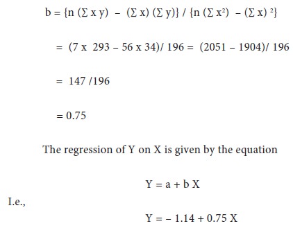
Y = a + b X ......................(1)
To find two quantities a and b, we require two equations. We have obtained one equation i.e., (2). We need one more equation. For this purpose, multiply both sides of (1) by
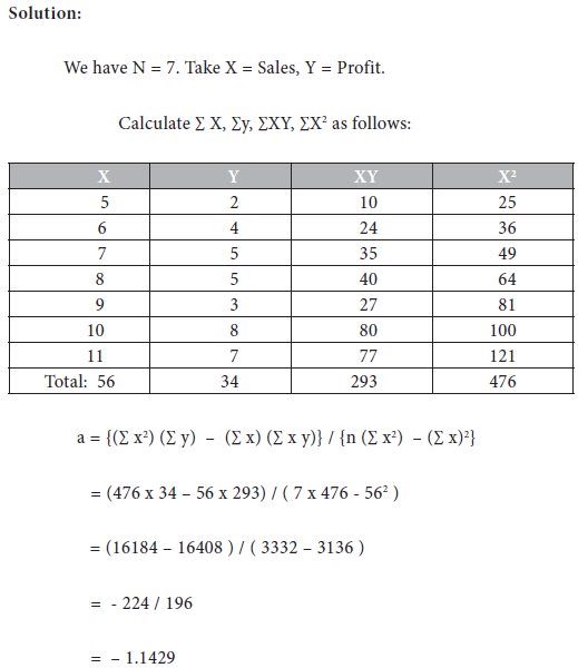
Problem 10
Consider the following data on sales and profit.
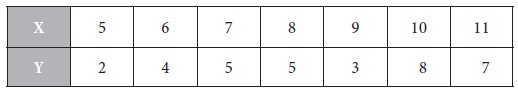
Determine the regression of profit on sales.
Problem 11
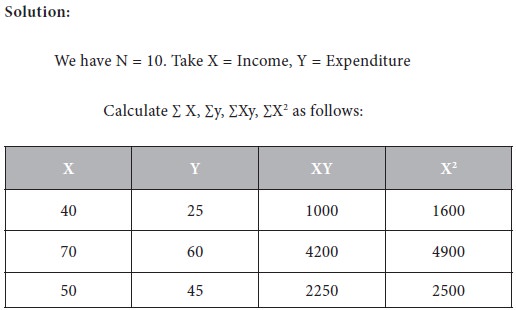
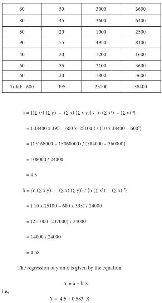
The following are the details of income and expenditure of 10 households.
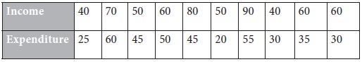
Determine the regression of expenditure on income and estimate the expenditure when the income is 65.
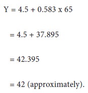
To estimate the expenditure when income is 65:
Take X = 65 in the above equation. Then we get
Problem 12
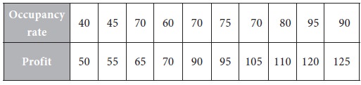
Consider the following data on occupancy rate and profit of a hotel.
Determine the regressions of
(i) profit on occupancy rate and
(ii) occupancy rate on profit.
Solution:
We have N = 10. Take X = Occupancy Rate, Y = Profit.
Note that in Problems 10 and 11, we wanted only one regression line and so we did not take ∑Y2 . Now we require two regression lines. Therefore,
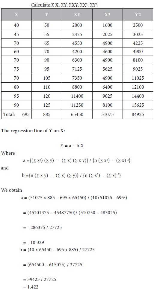
So, the regression equation is Y = - 10.329 + 1.422 X
Next, if we consider the regression line of X on Y, We get the equation X = a + b Y where
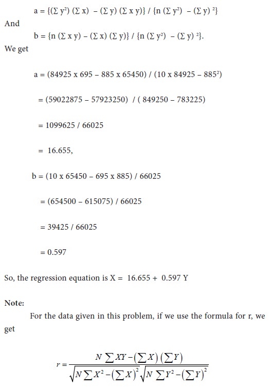
However, once we know the two b values, we can find the coefficient of correlation r between X and Y as the square root of the product of the two b values.Thus we obtain
Let x, y be two variables under consideration. Out of them, let x be an independent variable and let y be a dependent variable, depending on x. We desire to build a functional relationship between them. For this purpose, the first and foremost requirement is that x, y have a high degree of correlation. If the correlation coefficient between x and y is moderate or less, we shall not go ahead with the task of fitting a functional relationship between them.
Suppose there is a high degree of correlation (positive or negative) between x and y. Suppose it is required to build a linear relationship between them i.e., we want a regression of y on x.
Geometrically speaking, if we plot the corresponding values of x and y in a 2-dimensional plane and join such points, we shall obtain a straight line. However, hardly we can expect all the pairs (x, y) to lie on a straight line. We can consider several straight lines which are, to some extent, near all the points (x, y). Consider one line. An observation (x1, y1) may be either above the line of consideration or below the line. Project this point on the x-axis. It will meet the straight line at the point (x1, y1e). Here the theoretical value (or the expected value) of the variable is y1e while the observed value is y1. When there is a difference between the expected and observed values, there appears an error. This error is E1 = y1 –y1 . This is positive if (x1, y 1) is a point above the line and negative if (x1, y1) is a point below the line. For the n pairs of observations, we have the following n quantities of error:
Some of these quantities are positive while the remaining ones are negative. However, the squares of all these quantities are positive.
Among all those straight lines which are somewhat near to the given observations
we consider that straight line as the ideal one for which the sse is the least. Since the ideal straight line giving regression of y on x is based on this concept, we call this principle as the Principle of least squares.Normal equations
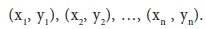
Suppose we have to fit a straight line to the n pairs of observations
Suppose the equation of straight line finally comes asY = a + b X ......................(1)
Where
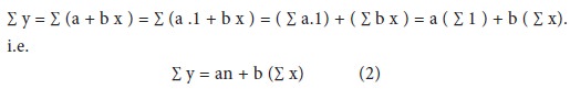
a, b are constants to be determined. Mathematically speaking, when we require finding the equation of a straight line, two distinct points on the straight line are sufficient. However, a different approach is followed here. We want to include all the observations in our attempt to build a straight line. Then all the n observed points (x, y) are required to satisfy the relation
(1). Consider the summation of all such terms. We get
To find two quantities a and b, we require two equations. We have obtained one equation i.e., (2). We need one more equation. For this purpose, multiply both sides of (1) by
x. We obtain
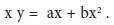
Consider the summation of all such terms. We get
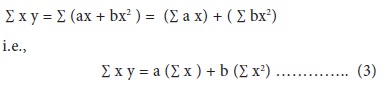
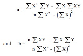
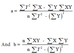
Equations (2) and (3) are referred to as the normal equations associated with the regression of y on x. Solving these two equations, we obtain
Note:
For calculating the coefficient of correlation,

For calculating the regression of y on x, we require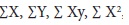 Thus, tabular column is same in both the cases with the difference that
  is also required for the coefficient of correlation.
Next, if we consider the regression line of x on y, we get the equation X = a + b y. The expressions for the coefficients can be got by interchanging the roles of X and Y in the previous discussion. Thus, we obtain
Consider the summation of all such terms. We get
Equations (2) and (3) are referred to as the normal equations associated with the regression of y on x. Solving these two equations, we obtain
Note:
For calculating the coefficient of correlation,
For calculating the regression of y on x, we require
Thus, tabular column is same in both the cases with the difference that Next, if we consider the regression line of x on y, we get the equation X = a + b y. The expressions for the coefficients can be got by interchanging the roles of X and Y in the previous discussion. Thus, we obtain
Problem 10
Consider the following data on sales and profit.
Determine the regression of profit on sales.
Problem 11
The following are the details of income and expenditure of 10 households.
Determine the regression of expenditure on income and estimate the expenditure when the income is 65.
To estimate the expenditure when income is 65:
Take X = 65 in the above equation. Then we get
Problem 12
Consider the following data on occupancy rate and profit of a hotel.
Determine the regressions of
(i) profit on occupancy rate and
(ii) occupancy rate on profit.
Solution:
We have N = 10. Take X = Occupancy Rate, Y = Profit.
Note that in Problems 10 and 11, we wanted only one regression line and so we did not take ∑Y2 . Now we require two regression lines. Therefore,
So, the regression equation is Y = - 10.329 + 1.422 X
Next, if we consider the regression line of X on Y, We get the equation X = a + b Y where
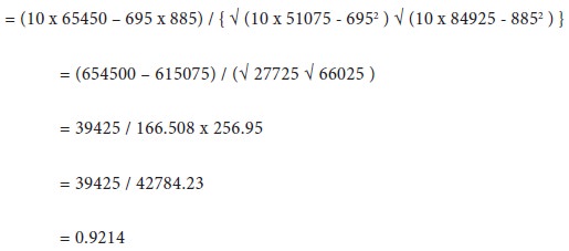
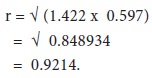
However, once we know the two b values, we can find the coefficient of correlation r between X and Y as the square root of the product of the two b values.Thus we obtain
Note that this agrees with the above value of r.
Tags : Research Methodology - Correlation And Regression Analysis
Last 30 days 1849 views