


Home | ARTS | Operations Management
|
Model I - Determining Economic Order Quantities-Deterministic Models – Purchase Order Quantities without shortages
Operations Management - Transportation / Assignment & Inventory Management
Model I - Determining Economic Order Quantities-Deterministic Models – Purchase Order Quantities without shortages
Posted On :
As we have already classified the economic order quantity or economic batch size problems into two types, based on the demand position.
Model I
Determination of the optimum quantity ordered (or produced) and the optimum interval between successive orders (or production) if the demand is known and uniform with no shortages permitted
An Illustration: Assume that you are required (as a student) Rs. 100/- to meet your daily requirements such as food, stay, refreshment etc. In a month, your demand is Rs. 3000/-. Whenever you are contacting parents, they are in a position to give your requirements in single stroke on the day itself. To get the money, you have to go to your native which costs you say Rs. 50/- Instead of keeping the money in your room, if you keep it in a bank, you may get an interest of Rs.20/- month. If this is the situation given to you, how much you have to get from your parents such that your holding/opportunity cost and ordering/procurement cost is, get balanced?
Here the problem is how much you have to get your parents every time so that the costs associated with holding the amount is get balanced? Here the example which may be seems to obvious, instead, if we take a car manufacturer, whose requirement is say 3000 Gear boxes per month, who is producing 100 cars in a day, finds that, keeping a gear box in warehouse costs him Rs. 200/- per month (excluding cost of gear box) and placing the order would costs Rs. 500 per order. In this situation, how much gear boxes he has to order, how much should be the order size so that the cost
If we summarize the assumptions, we are approaching the problems through Economic Order Quantity or Economic Lot Size problems, or in general known as EOQ problems.
Solution
Let us make the following assumptions:
1. Let the demand is known and uniform. Let D be the demand for a period say 1-year.
2.
Shortages
are not permitted.
3. Let the replenishment of items be instantaneous.
4. Lead-time is zero.
5. Let Q be the Economic Order Quantity for every cycle.
6. Let Cs be the Set up cost for every cycle
7. Let C1 be the inventory holding cost per unit per unit of time.
Let us divide the one-year into n equal parts each of duration‘t’
Therefore n * t = 1 or t = 1/n
Let Q be the economic order quantity for every cycle.
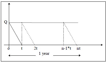
The graph of this model is given by,
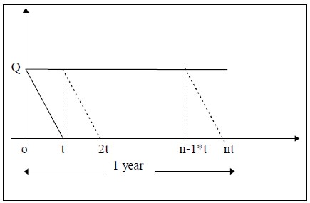
Therefore n * Q = D or
t = Q/D
Inventory for the time period t = Area of the triangle Qot
= ½ t* Q
Therefore the Average inventory for one unit of time
= [½ t *Q]/ t = Q/2
Since all the triangles are similar, the average inventory for the whole year = ½ Q
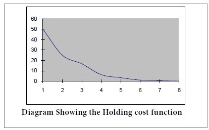
Therefore the annual inventory holding cost = ½ Q * C1 -------- (1)
In addition, Ca is a function on Q. For maximization or minimization, the first derivative is found out and equated with zero. If the second derivative is greater than zero indicates the function attains its
Moreover, the second derivative is strictly greater than zero.
By substituting the value of Q, which has derived just now, which is possessing the characteristic of balancing the ordering cost and holding cost, in the equation for total cost function Ca, we get
Case 1
Let us assume that the year we divided into n parts say, t1, t2, t3, etc., which are not equal.
The total inventory over time t1 = ½ Q * t1
Total inventory over time t2 = ½ Q * t2 and so on.
Therefore total inventory over 1 year = ½ Q * [t1 + t2 + … +tn] = ½ Q * t
And Average inventory = ½Q
Therefore Annual inventory holding cost = ½ Q * C1
Since annual set up cost is the same, we will get the same Ca hence; we will get the same EOQ and other related issues.
Therefore,
E.O.Q = [2 * D * Cs / C1] ½
n = D/Q
And t = 1/n
Case 2
Let the Setup cost depend on the # of units that are being ordered or produced.
Since the set up cost for a cycle = Cs + Q * b, where ‘b’ is the cost of ordering one unit.
Therefore Ca = [½ * Q* C1] + D/Q (Cs + Q *b)
And d (Ca)/ d Q = 0 implies,
d (Ca)/ d Q = ½ C1 - DCs/ Q2 =0
Or D
* Cs / Q2 = ½ C1
Q2 = 2 * D * Cs / C1
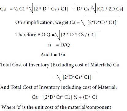
Q = [2 * D * Cs / C1] ½
And, Ca = ½ C1 * [2 * D * Cs / C1] ½ + D* Cs *[C1 / 2D Cs] ½ + D* b
On
simplification, we get Ca = [2*D*Cs* C1] ½ + D* b
Example-3

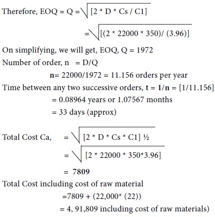
Preethi Computers purchases 22,000 silicon chips every year and each unit cost Rs. 22/-, as they are purchasing in bulk quantity such a low price is possible. Cost of each order is Rs. 350/-. Its inventory carrying cost is 18% of average inventory. What should be EOQ. What is the optimum number of day’s supply for optimum order? What is the annual cost on inventory including cost of the material?
Solution
From the given problem, it is clear that,
Example-4
PRG Engineering Company is a distributor for water pumps. The company’s sales amount to 50,000 units of Water Pumps per year. The order receiving/processing and handling cost are Rs. 3 per order while the trucking cost is Rs. 12 per order. Further, the interest cost is Rs. 0.06 per unit per year. Deterioration cost is Rs. 0.004 per unit per year. Storage cost is Rs. 1000/year for 50000 units. Find the EOQ; also find the time between orders and number of orders to be placed.
Solution
From the given problem, it is clear that,
Demand, D = 50000 pumps /year
Carrying cost, C1 = 0.006 + 0.004 + 1000/50000 = 0.084
Cost of set up, Cs = Rs. 3+5= 15 per order
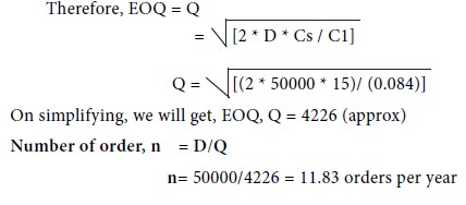
Time between any two successive orders, t = 1/n = [1/11.83]
= 0.08452 years or 1.01424 months
= 30.427 days (approx)
Determination of the optimum quantity ordered (or produced) and the optimum interval between successive orders (or production) if the demand is known and uniform with no shortages permitted
An Illustration: Assume that you are required (as a student) Rs. 100/- to meet your daily requirements such as food, stay, refreshment etc. In a month, your demand is Rs. 3000/-. Whenever you are contacting parents, they are in a position to give your requirements in single stroke on the day itself. To get the money, you have to go to your native which costs you say Rs. 50/- Instead of keeping the money in your room, if you keep it in a bank, you may get an interest of Rs.20/- month. If this is the situation given to you, how much you have to get from your parents such that your holding/opportunity cost and ordering/procurement cost is, get balanced?
Here the problem is how much you have to get your parents every time so that the costs associated with holding the amount is get balanced? Here the example which may be seems to obvious, instead, if we take a car manufacturer, whose requirement is say 3000 Gear boxes per month, who is producing 100 cars in a day, finds that, keeping a gear box in warehouse costs him Rs. 200/- per month (excluding cost of gear box) and placing the order would costs Rs. 500 per order. In this situation, how much gear boxes he has to order, how much should be the order size so that the cost
If we summarize the assumptions, we are approaching the problems through Economic Order Quantity or Economic Lot Size problems, or in general known as EOQ problems.
Solution
Let us make the following assumptions:
1. Let the demand is known and uniform. Let D be the demand for a period say 1-year.
3. Let the replenishment of items be instantaneous.
4. Lead-time is zero.
5. Let Q be the Economic Order Quantity for every cycle.
6. Let Cs be the Set up cost for every cycle
7. Let C1 be the inventory holding cost per unit per unit of time.
Let us divide the one-year into n equal parts each of duration‘t’
Therefore n * t = 1 or t = 1/n
Let Q be the economic order quantity for every cycle.
The graph of this model is given by,
Therefore n * Q = D or
t = Q/D
Inventory for the time period t = Area of the triangle Qot
= ½ t* Q
Therefore the Average inventory for one unit of time
= [½ t *Q]/ t = Q/2
Since all the triangles are similar, the average inventory for the whole year = ½ Q
Therefore the annual inventory holding cost = ½ Q * C1 -------- (1)
And
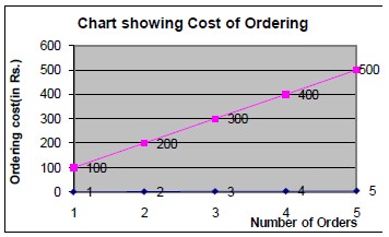
Annual Set up cost | = | n * Cs | ---------
(2) | ||||||||||
= D/Q *
Cs | (since
n * Q = D) |
| |||||||||||
Therefore Annual Total Cost Ca = ½ Q * C1 + D/Q * Cs ---- | (3) |
In addition, Ca is a function on Q. For maximization or minimization, the first derivative is found out and equated with zero. If the second derivative is greater than zero indicates the function attains its
Moreover, the second derivative is strictly greater than zero.
By substituting the value of Q, which has derived just now, which is possessing the characteristic of balancing the ordering cost and holding cost, in the equation for total cost function Ca, we get
Some Special Cases
Case 1
Let us assume that the year we divided into n parts say, t1, t2, t3, etc., which are not equal.
The total inventory over time t1 = ½ Q * t1
Total inventory over time t2 = ½ Q * t2 and so on.
Therefore total inventory over 1 year = ½ Q * [t1 + t2 + … +tn] = ½ Q * t
And Average inventory = ½Q
Therefore Annual inventory holding cost = ½ Q * C1
Since annual set up cost is the same, we will get the same Ca hence; we will get the same EOQ and other related issues.
Therefore,
E.O.Q = [2 * D * Cs / C1] ½
n = D/Q
And t = 1/n
Case 2
Let the Setup cost depend on the # of units that are being ordered or produced.
Since the set up cost for a cycle = Cs + Q * b, where ‘b’ is the cost of ordering one unit.
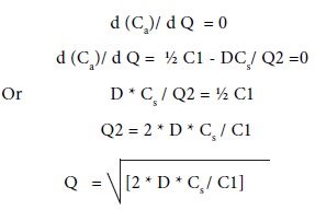
Therefore Ca = [½ * Q* C1] + D/Q (Cs + Q *b)
And d (Ca)/ d Q = 0 implies,
d (Ca)/ d Q = ½ C1 - DCs/ Q2 =0
Q2 = 2 * D * Cs / C1
Q = [2 * D * Cs / C1] ½
And, Ca = ½ C1 * [2 * D * Cs / C1] ½ + D* Cs *[C1 / 2D Cs] ½ + D* b
Note: The only change is addition of D*b term in the cost.
Example-1
SMS Limited uses annually 24,000 Paper Boxes, which costs Rs. 1.25/- per unit. Placing each order cost Rs. 22.50/- and the carrying cost is 5.4% per year of the average inventory. Find the total cost including the cost of Boxes.
Solution
D = 24,000 Cs = Rs. 22.50/-
And C1 = 1.25 * 5.4% = 0.0675/Boxes/year.
Therefore, EOQ, Q = [2 * D * Cs / C1] ½ = 4000 Boxes And ‘n’ = D/Q = 24000/ 4000 = 6 i.e. we have to make 6 orders
t = Q/D
= 4000/24000
= 0.16666 years or
= 0.16666* 12
= 2 months
Total Cost Ca, = [2 * D * Cs * C1] ½
= 270/-
Total Cost including cost of raw material = 270 + [24000 * 1.25] = 30270/-
Example-2
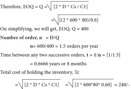
M/s Shriram Industries has to supply 600 industrial fans per year. The firm never permitted shortages to occur. Moreover, the storage cost amounts to Rs. 0.60/ unit/ year. The set up cost per production run is Rs. 80/-. Find the optimum order quantity, number of orders to place in a year and average yearly cost.
Solution
From the given problem, it is clear that,
Demand, D = 600 units/year
Carrying cost, C1 = 0.60/unit/year
Cost of set up, Cs = Rs. 80/-
Example-1
SMS Limited uses annually 24,000 Paper Boxes, which costs Rs. 1.25/- per unit. Placing each order cost Rs. 22.50/- and the carrying cost is 5.4% per year of the average inventory. Find the total cost including the cost of Boxes.
Solution
D = 24,000 Cs = Rs. 22.50/-
And C1 = 1.25 * 5.4% = 0.0675/Boxes/year.
Therefore, EOQ, Q = [2 * D * Cs / C1] ½ = 4000 Boxes And ‘n’ = D/Q = 24000/ 4000 = 6 i.e. we have to make 6 orders
t = Q/D
= 4000/24000
= 0.16666 years or
= 0.16666* 12
= 2 months
Total Cost Ca, = [2 * D * Cs * C1] ½
= 270/-
Total Cost including cost of raw material = 270 + [24000 * 1.25] = 30270/-
Example-2
M/s Shriram Industries has to supply 600 industrial fans per year. The firm never permitted shortages to occur. Moreover, the storage cost amounts to Rs. 0.60/ unit/ year. The set up cost per production run is Rs. 80/-. Find the optimum order quantity, number of orders to place in a year and average yearly cost.
Solution
From the given problem, it is clear that,
Demand, D = 600 units/year
Carrying cost, C1 = 0.60/unit/year
Cost of set up, Cs = Rs. 80/-
Example-3
Preethi Computers purchases 22,000 silicon chips every year and each unit cost Rs. 22/-, as they are purchasing in bulk quantity such a low price is possible. Cost of each order is Rs. 350/-. Its inventory carrying cost is 18% of average inventory. What should be EOQ. What is the optimum number of day’s supply for optimum order? What is the annual cost on inventory including cost of the material?
Solution
From the given problem, it is clear that,
Demand, | D = 22000 units/year | |||
Cost of material, | C= Rs. 22 per unit | |||
Carrying cost, | C1 =
18% * (22) = 3.96 | |||
Cost of set up, | Cs = Rs. 350/- | |||
Example-4
PRG Engineering Company is a distributor for water pumps. The company’s sales amount to 50,000 units of Water Pumps per year. The order receiving/processing and handling cost are Rs. 3 per order while the trucking cost is Rs. 12 per order. Further, the interest cost is Rs. 0.06 per unit per year. Deterioration cost is Rs. 0.004 per unit per year. Storage cost is Rs. 1000/year for 50000 units. Find the EOQ; also find the time between orders and number of orders to be placed.
Solution
From the given problem, it is clear that,
Demand, D = 50000 pumps /year
Carrying cost, C1 = 0.006 + 0.004 + 1000/50000 = 0.084
Cost of set up, Cs = Rs. 3+5= 15 per order
Time between any two successive orders, t = 1/n = [1/11.83]
= 0.08452 years or 1.01424 months
= 30.427 days (approx)
Tags : Operations Management - Transportation / Assignment & Inventory Management
Last 30 days 953 views