


Research Methodology - Analysis Of Variance
ANOVA for One-way classified data
Posted On :
Let y denote the jth observation corresponding to the ith level of factor A and Yij the corresponding random variate.
ANOVA for
One-way classified data
Let y denote the jth observation corresponding to the ith level of factor A and Yij the corresponding random variate.
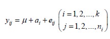
Define the linear model for the sample data obtained from the experiment by the equation
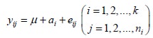
Where µ represents the general mean effect which is fixed and which represents the general condition of the experimental units, ai denotes the fixed effect due to ith level of the factor A (i=1,2,…,k) and hence the variation due to ai (i=1,2,…,k) is said to be control.
The last component of the model eij is the random variable. It is called the error component and it makes the Yij a random variate. The variation in eij is due to all the uncontrolled factors and eij is independently, identically and normally distributed with mean zero and constant variance σ2 .
For the realization of the random variate Yij, consider yij defined by
The expected value of the general observation yij in the experimental units is given by
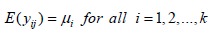
With yij=µi+eij , where eij is the random error effect due to uncontrolled factors (i.e., due to chance only).
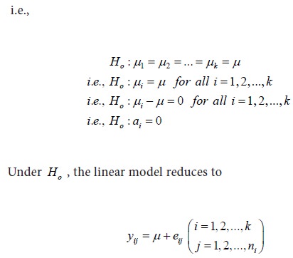
Here we may expect µi=µ for all i=1,2,....,k , if there is no variation due to control factors. If it is not the case, we have
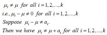
On substitution for µi in the above equation, the linear model reduces to
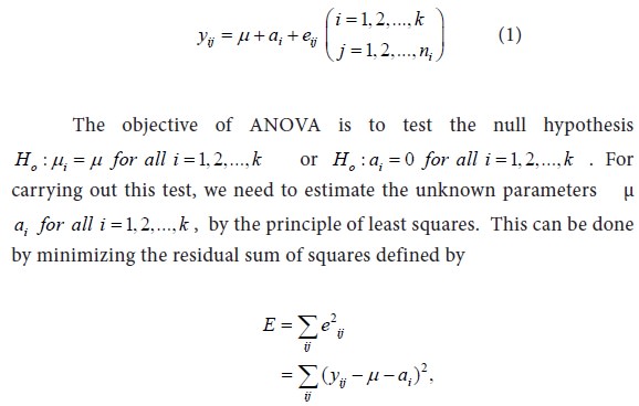
Using (1). The normal equations can be obtained by partially differentiating E with respect to µ and ai for all i = 1, 2,..., k and equating the results to zero. We obtain
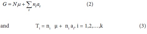
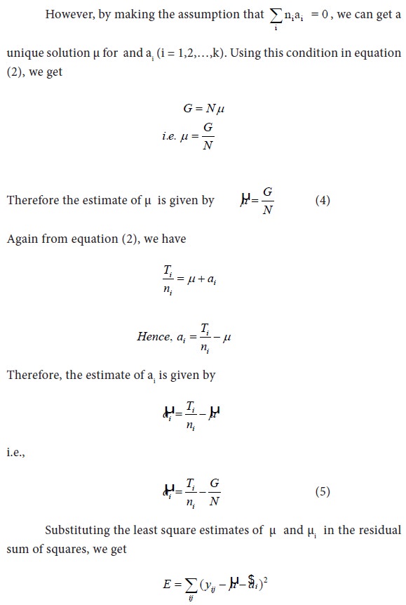
Where N = nk. We see that the number of variables (k+1) is more than the number of independent equations (k). So, by the theorem on a system of linear equations, it follows that unique solution for this system is not possible.
After carrying out some calculations and using the normal equations (2) and (3) we obtain
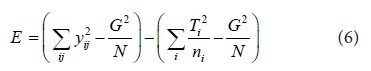
The first term in the RHS of equation (6) is called the corrected total sum of squares while is called the uncorrected
total sum of squares.
is called the uncorrected
total sum of squares.
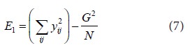
Proceeding as before, we get the residual sum of squares for this hypothetical model as
Actually, E1 contains the variation due to both treatment and error. Therefore a measure of variation due to treatment can be obtained by “ E1 − E ”. Using (6) and (7), we get
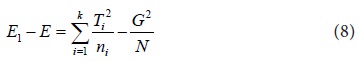
The expression in (8) is usually called the corrected treatment sum of squares while the term is called uncorrected treatment sum of
squares. Here it may be noted that
is called uncorrected treatment sum of
squares. Here it may be noted that  is a correction factor (also called a correction term). Since E is based on N-K
free observations, it has N - K degrees of freedom (df). Similarly, since E1 is
based on N -1 free observation, E1
has N -1 degrees of freedom. So E1 − E has K -1 degrees of freedom.
is a correction factor (also called a correction term). Since E is based on N-K
free observations, it has N - K degrees of freedom (df). Similarly, since E1 is
based on N -1 free observation, E1
has N -1 degrees of freedom. So E1 − E has K -1 degrees of freedom.
Let y denote the jth observation corresponding to the ith level of factor A and Yij the corresponding random variate.
Define the linear model for the sample data obtained from the experiment by the equation
Where µ represents the general mean effect which is fixed and which represents the general condition of the experimental units, ai denotes the fixed effect due to ith level of the factor A (i=1,2,…,k) and hence the variation due to ai (i=1,2,…,k) is said to be control.
The last component of the model eij is the random variable. It is called the error component and it makes the Yij a random variate. The variation in eij is due to all the uncontrolled factors and eij is independently, identically and normally distributed with mean zero and constant variance σ2 .
For the realization of the random variate Yij, consider yij defined by
The expected value of the general observation yij in the experimental units is given by
With yij=µi+eij , where eij is the random error effect due to uncontrolled factors (i.e., due to chance only).
Here we may expect µi=µ for all i=1,2,....,k , if there is no variation due to control factors. If it is not the case, we have
On substitution for µi in the above equation, the linear model reduces to
Using (1). The normal equations can be obtained by partially differentiating E with respect to µ and ai for all i = 1, 2,..., k and equating the results to zero. We obtain
Where N = nk. We see that the number of variables (k+1) is more than the number of independent equations (k). So, by the theorem on a system of linear equations, it follows that unique solution for this system is not possible.
After carrying out some calculations and using the normal equations (2) and (3) we obtain
The first term in the RHS of equation (6) is called the corrected total sum of squares while
for measuring the variation due to treatment (controlled
factor), we consider the null hypothesis that all the treatment effects are
equal.
Proceeding as before, we get the residual sum of squares for this hypothetical model as
Actually, E1 contains the variation due to both treatment and error. Therefore a measure of variation due to treatment can be obtained by “ E1 − E ”. Using (6) and (7), we get
The expression in (8) is usually called the corrected treatment sum of squares while the term
When actually the null hypothesis is true, if we
reject it on the basis of the estimated value in our statistical analysis, we
will be committing Type – I Error.
The probability for committing this error is referred to as the denoted by α. The
testing of the null hypothesis Ho
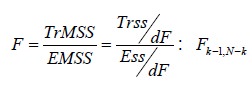
may be carried out by F test. For given α,
we have
i.e., It follows F distribution with degrees of
freedom K-1 and N-K.
Tags : Research Methodology - Analysis Of Variance
Last 30 days 984 views