


Home | ARTS | Financial Management
|
Risk and Uncertainty incorporated methods of Capital Project evaluation - Risk Analysis In Capital Budgeting
Financial Management - Capital Budgeting – A Conceptual Framework
Risk and Uncertainty incorporated methods of Capital Project evaluation - Risk Analysis In Capital Budgeting
Posted On :
Risk with reference to capital (budgeting) investment decisions may be defined as the variability which is likely to occur in future between estimated return and actual return. Uncertainty is total lack of ability to pinpoint expected return.
Risk and Uncertainty incorporated methods of
Capital Project evaluation
Risk with reference to capital (budgeting) investment decisions may be defined as the variability which is likely to occur in future between estimated return and actual return. Uncertainty is total lack of ability to pinpoint expected return.
Situations of pure risk refer to contingencies which have to be protected against the normal insurance practice of pooling. For this to be so, risk situations are characterized by a considerable degree of past experience. Uncertainty on the other hand relates to situations in some sense unique and of which there is very little certain knowledge of some or all significant aspects.
The techniques used to handle risk may be classified into the groups as follows:
(a) Conservative methods
These methods include shorter payback period, risk-adjusted discount rate, and conservative forecasts or certainty equivalents etc., and
(b) Modern methods
They include sensitivity analysis, probability analysis, decision-tree analysis etc.
The conservative methods of risk handling are dealt with now.
According to this method, projects with shorter payback period are normally preferred to those with longer payback period. It would be more effective when it is combined with “cut off period”. Cut off period denotes the risk tolerance level of the firms. For example, a firm has three projects. A , B and C for consideration with different economic lives say 15,16 and 18 years respectively and with payback periods of say 6, 7 and 5 years. Of these three, project C will be preferred, for its payback period is the shortest. Suppose, the cut off period is 4 years, .then all the three projects will be rejected.
Risk Adjusted Discount Rate is based on the same logic as the net present value method. Under this method, discount rate is adjusted in accordance with the degree of risk. That is, a risk discount factor (known as risk-premium rate) is determined and added to the discount factor (risk free rate) otherwise used for calculating net present value. For example, the rate of interest (r) employed in the discounting is 10 per cent and the risk discount factor or degrees of risk (d) are 2, 4 and 5 per cent for mildly risky, moderately risky and high risk (or speculative) projects respectively then the total rate of discount (D) would respectively be 12 per cent, 14 per cent and 15 .per cent.
That is RADR = 1/ (8+r+d). The idea is the greater the risk the higher the discount rate. That is, for the first year the total discount factor, D= 1 / (1+r+d) for the second year RADR = 1 / (1+r+d) 2 and so on.
Normally, risk discount factor would vary from project to project depending upon the quantum of risk. It is estimated on the basis of judgment and intention on the part of management, which in turn are subject to risk attitude of management.
It may be noted that the higher the risk, the higher the risk adjusted discount rate, and the lower the discounted present value. The Risk Adjusted Discount Rate is composite of discount rate which combines .both time and risk factors.
Risk Adjusted Discount Rate can be used with both NPV and LRX. In the case of NPV future cash flows should be discounted using Risk Adjusted Discount Rate and then NPV may be ascertained. If the NPV were positive, the project would qualify for acceptance. A negative NPV would signify that the project should be rejected. If LRR method were used, the IRR would be computed and compared “with the modified discount rate. If it, exceeds modified discount rate, the proposal would be accepted, otherwise rejected.
1. This technique is simple and easy to handle in practice.
2. The discount rates can be adjusted for the varying degrees of risk in different years, simply by increasing or decreasing the risk factor (d) in calculating the risk adjusted discount rate.
3. This method of discounting is such that the higher the risk factor in the remote future is, automatically accounted for. The risk adjusted discount rate is a composite rate which combines both the time and discount factors.
i) The value of discount factor must necessarily remain subjective as it is primarily based on investor’s attitude towards risk. .
ii) A uniform risk discount factor used for discounting al future returns is unscientific as it implies the risk level of investment remains same over the years where as in practice is not so.
This risk element in any decision is often characterized by the two Outcomes: the ‘potential gain’ at the one end and the ‘potential loss’ at the other. These are respectively called the focal gain and focal loss. In this connection, Shackle proposes the concept of “potential surprise” which is a unit of measurement indicating the decision-maker’s surprise at the occurrence of an event other than what he was expecting. He also introduces “another concept - the “certainty equivalent” of risky investment. For an investment X with a given degree of risk, investor can always find another risk less investment Xi such that he is indifferent between X arid Xi. The difference between X and Xi is implicitly the risk discount.
The risk level of the project under this method is taken into account by adjusting the expected cash inflows and the discount rate. Thus the expected cash inflows are reduced to a conservative level by risk-adjustment factor (also called correction factor). This factor is expressed in terms of Certainty - Equivalent Co-efficient which is the ratio of risk less cash flows to risky cash lows. Thus Certainty — Equivalent Co-efficient;
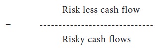
This co-efficient is calculated for cash flows of each year. The value of the co-efficient may vary-between 0 and 1, there is inverse relationship between the degree of risk, and the value of co-efficient computed.
These adjusted cash inflows are used for calculating N.P.V. and the I.R.R. The discount rate to be used for calculating present values will be risk-free (i.e., the rate reflecting the time value of money). Using this criterion of the N.P.V. the project would be accepted, if the N.P.V were positive, otherwise it would be rejected. The I.R.R. will be compared with risk free discount rate and if it higher the project will be accepted, otherwise rejected.
This method is similar to payback method applied under the condition of certainty. In this method, a terminal data is fixed. In the decision making, only the expected returns or gain prior to the terminal data are considered. The gains or benefit expected beyond the terminal data are ignored the gains are simply treated as non-existent. The logic behind this approach is that the developments during the period under Consideration might render the gains beyond terminal date of no consequence. For example, a Hyde project might go out of use, when, say, after 50-years, of its installation, the atomic or solar energy becomes available in abundance and at lower cost.
This provides information about cash flows under three assumptions: i) pessimistic, ii) most likely and iii) optimistic outcomes associated with the project. It is superior to one figure forecast as it gives a more precise idea about the variability of the return. This explains how sensitive the cash flows or under the above mentioned different situations. The larger is the difference between the pessimistic and optimistic cash flows, the more risky is the project.
Decision tree analysis is another technique which is helpful in tackling risky capital investment proposals. Decision tree is a graphic display of relationship between a present decision and possible future events, future decisions and their consequence. The sequence of event is mapped out over time in a format resembling branches of a tree. In other words, it is pictorial representation in tree from which indicates the magnitude probability and inter-relationship of all possible outcomes.
Managerial Economics focuses attention on the development of tools for finding out an optimal or best solution for the specified objectives in business. Any decision has the following elements:
Project risk refers to fluctuation in its payback period, ARR, IRR, NPV or so. Higher the fluctuation, higher is the risk and vice versa. Let us take NPV based risk.
If NPV from year to year fluctuate, there is risk. This can be measured through standard deviation of the NPV figures. Suppose the expected NPV of a project is Rs. 18 lakhs, and std.’-deviation of Rs. 6 lakhs. The coefficient of variation C V is given by std. deviation divided by NPV.
C, V = Rs. 6,00,000 / ` 18,00,000 = 0.33
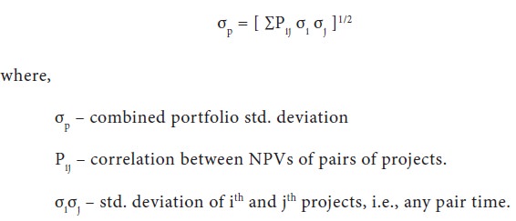
When multiple projects are
considered together, what is the overall risk of all projects put together? Is
it the aggregate average of std. deviation of NPV of all projects? No, it is
not. Then What? Now another variable has to be brought to the scene. That is
the correlation coefficient between NPVs of pairs of projects. When two
projects are considered together, the variation in the combined NPV is
influenced by the extent of correlation between NPVs of the projects in
question. A high correlation results in high risk and vice versa. So, the risk
of all projects put together in the form ‘of combined std. deviation is given
by the formula:
Risk with reference to capital (budgeting) investment decisions may be defined as the variability which is likely to occur in future between estimated return and actual return. Uncertainty is total lack of ability to pinpoint expected return.
Situations of pure risk refer to contingencies which have to be protected against the normal insurance practice of pooling. For this to be so, risk situations are characterized by a considerable degree of past experience. Uncertainty on the other hand relates to situations in some sense unique and of which there is very little certain knowledge of some or all significant aspects.
The techniques used to handle risk may be classified into the groups as follows:
(a) Conservative methods
These methods include shorter payback period, risk-adjusted discount rate, and conservative forecasts or certainty equivalents etc., and
(b) Modern methods
They include sensitivity analysis, probability analysis, decision-tree analysis etc.
i. Conservative Methods
The conservative methods of risk handling are dealt with now.
1. Shorter Payback Period
According to this method, projects with shorter payback period are normally preferred to those with longer payback period. It would be more effective when it is combined with “cut off period”. Cut off period denotes the risk tolerance level of the firms. For example, a firm has three projects. A , B and C for consideration with different economic lives say 15,16 and 18 years respectively and with payback periods of say 6, 7 and 5 years. Of these three, project C will be preferred, for its payback period is the shortest. Suppose, the cut off period is 4 years, .then all the three projects will be rejected.
2. Risk
Adjusted Discount Rate (RADR)
Risk Adjusted Discount Rate is based on the same logic as the net present value method. Under this method, discount rate is adjusted in accordance with the degree of risk. That is, a risk discount factor (known as risk-premium rate) is determined and added to the discount factor (risk free rate) otherwise used for calculating net present value. For example, the rate of interest (r) employed in the discounting is 10 per cent and the risk discount factor or degrees of risk (d) are 2, 4 and 5 per cent for mildly risky, moderately risky and high risk (or speculative) projects respectively then the total rate of discount (D) would respectively be 12 per cent, 14 per cent and 15 .per cent.
That is RADR = 1/ (8+r+d). The idea is the greater the risk the higher the discount rate. That is, for the first year the total discount factor, D= 1 / (1+r+d) for the second year RADR = 1 / (1+r+d) 2 and so on.
Normally, risk discount factor would vary from project to project depending upon the quantum of risk. It is estimated on the basis of judgment and intention on the part of management, which in turn are subject to risk attitude of management.
It may be noted that the higher the risk, the higher the risk adjusted discount rate, and the lower the discounted present value. The Risk Adjusted Discount Rate is composite of discount rate which combines .both time and risk factors.
Risk Adjusted Discount Rate can be used with both NPV and LRX. In the case of NPV future cash flows should be discounted using Risk Adjusted Discount Rate and then NPV may be ascertained. If the NPV were positive, the project would qualify for acceptance. A negative NPV would signify that the project should be rejected. If LRR method were used, the IRR would be computed and compared “with the modified discount rate. If it, exceeds modified discount rate, the proposal would be accepted, otherwise rejected.
Risk Adjusted Discount Rate Method – Merits:
1. This technique is simple and easy to handle in practice.
2. The discount rates can be adjusted for the varying degrees of risk in different years, simply by increasing or decreasing the risk factor (d) in calculating the risk adjusted discount rate.
3. This method of discounting is such that the higher the risk factor in the remote future is, automatically accounted for. The risk adjusted discount rate is a composite rate which combines both the time and discount factors.
Risk Adjusted Discount Rate Method – Demerits:
i) The value of discount factor must necessarily remain subjective as it is primarily based on investor’s attitude towards risk. .
ii) A uniform risk discount factor used for discounting al future returns is unscientific as it implies the risk level of investment remains same over the years where as in practice is not so.
Certainty-Equivalent Coefficient Approach
This risk element in any decision is often characterized by the two Outcomes: the ‘potential gain’ at the one end and the ‘potential loss’ at the other. These are respectively called the focal gain and focal loss. In this connection, Shackle proposes the concept of “potential surprise” which is a unit of measurement indicating the decision-maker’s surprise at the occurrence of an event other than what he was expecting. He also introduces “another concept - the “certainty equivalent” of risky investment. For an investment X with a given degree of risk, investor can always find another risk less investment Xi such that he is indifferent between X arid Xi. The difference between X and Xi is implicitly the risk discount.
The risk level of the project under this method is taken into account by adjusting the expected cash inflows and the discount rate. Thus the expected cash inflows are reduced to a conservative level by risk-adjustment factor (also called correction factor). This factor is expressed in terms of Certainty - Equivalent Co-efficient which is the ratio of risk less cash flows to risky cash lows. Thus Certainty — Equivalent Co-efficient;
This co-efficient is calculated for cash flows of each year. The value of the co-efficient may vary-between 0 and 1, there is inverse relationship between the degree of risk, and the value of co-efficient computed.
These adjusted cash inflows are used for calculating N.P.V. and the I.R.R. The discount rate to be used for calculating present values will be risk-free (i.e., the rate reflecting the time value of money). Using this criterion of the N.P.V. the project would be accepted, if the N.P.V were positive, otherwise it would be rejected. The I.R.R. will be compared with risk free discount rate and if it higher the project will be accepted, otherwise rejected.
The Finite-horizon Method
This method is similar to payback method applied under the condition of certainty. In this method, a terminal data is fixed. In the decision making, only the expected returns or gain prior to the terminal data are considered. The gains or benefit expected beyond the terminal data are ignored the gains are simply treated as non-existent. The logic behind this approach is that the developments during the period under Consideration might render the gains beyond terminal date of no consequence. For example, a Hyde project might go out of use, when, say, after 50-years, of its installation, the atomic or solar energy becomes available in abundance and at lower cost.
ii.Modern Methods
Sensitivity Analysis
This provides information about cash flows under three assumptions: i) pessimistic, ii) most likely and iii) optimistic outcomes associated with the project. It is superior to one figure forecast as it gives a more precise idea about the variability of the return. This explains how sensitive the cash flows or under the above mentioned different situations. The larger is the difference between the pessimistic and optimistic cash flows, the more risky is the project.
Decision Tree Analysis
Decision tree analysis is another technique which is helpful in tackling risky capital investment proposals. Decision tree is a graphic display of relationship between a present decision and possible future events, future decisions and their consequence. The sequence of event is mapped out over time in a format resembling branches of a tree. In other words, it is pictorial representation in tree from which indicates the magnitude probability and inter-relationship of all possible outcomes.
Elements of Decision Theory
Managerial Economics focuses attention on the development of tools for finding out an optimal or best solution for the specified objectives in business. Any decision has the following elements:
1. The Decision Maker.
2. Objectives or goals sought to be achieved by the decision maker; for example, maximisation of profit or sales revenue may be the objective of the business
3. A set of choice alternatives, for example the available projects in Capital budgeting.
4. A set of outcomes or pay-offs with each alternatives; that is net benefits from the projects. Outcomes may be certain or uncertain. In case of former, the selection of any alternative leads uniquely to a specific pay-off. In case of later, any one of a number of outcomes may be associated with any specific decision.
5. A number of states of the environment whose occurrence determines the possible outcomes. For example, inflation and depression would be two alternative states, in the absence of risk and uncertainty, the outcome of a project is known. Therefore only one state of the environment is possible. The study of Managerial Economics begins with developing awareness of the environment within which managerial decisions are made.
6. Criteria derived from the general objectives which enable the decision taker to rank the various alternatives in terms of how far their pay-offs lead to the achievement of the decision maker’s goals. This is known as the decision process.
7. Constraints on the alternatives when the decision maker may select. For example, the government policy on monopoly control; top management directions regarding business undertakings, diversification of business or diversifying an existing product line or to refrain from certain types of business, etc.
Risk Analysis in the case of Single Project
Project risk refers to fluctuation in its payback period, ARR, IRR, NPV or so. Higher the fluctuation, higher is the risk and vice versa. Let us take NPV based risk.
If NPV from year to year fluctuate, there is risk. This can be measured through standard deviation of the NPV figures. Suppose the expected NPV of a project is Rs. 18 lakhs, and std.’-deviation of Rs. 6 lakhs. The coefficient of variation C V is given by std. deviation divided by NPV.
C, V = Rs. 6,00,000 / ` 18,00,000 = 0.33
Risk Return Analysis for Multi Projects
Tags : Financial Management - Capital Budgeting – A Conceptual Framework
Last 30 days 2464 views