


Operations Management - Game Theory, Goal Programming & Queuing Theory
Types of Waiting Line Models - Queueing Theory
Posted On :
In general, a queueing model can be classified into six categories using Kendall’s notation with six parameters to define a model. The parameters of this notation are as follows.
Types of
Waiting Line Models
In general, a queueing model can be classified into six categories using Kendall’s notation with six parameters to define a model. The parameters of this notation are as follows.
P- Arrival rate distribution i.e probability law for the arrival /inter – arrival time.
Q - Service rate distribution, i.e probability law according to which the customers are being served
R - Number of Servers (i.e., number of service points)
X - Service discipline
Y - Maximum number of customers allowed in the system
Z - Size of the calling source of the customers
A queuing model with the above parameters is denoted by the symbol (P/Q/R : X/Y/Z)
This is a waiting line model with the following properties:
1. The arrival rate follows Poisson (M) distribution
2. The service rate follows Poisson distribution (M)
3. The number of servers in the system is 1
4. The service discipline is general discipline (i.e., GD)
5. Maximum number of customers allowed in the system is infinite (∞)
6. he size of the calling source is infinite (∞)
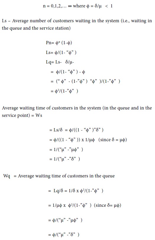
The steady state equations to obtain Pn, the probability of having n customers in the system, and the formulae for obtaining the values for Ls, Lq, Ws and Wq are as follows:
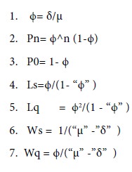
Summary of Formulae
Example 1
The arrival rate of customers at a petrol bunk follows a Poisson distribution with a mean of 27 per hour. The petrol bunk has only one unit of service. The service rate at the petrol bunk also follows Poisson distribution with mean of 36 per hour. Determine the following:
What is the probability of having zero customer in the system ?
Note: In the determination of Ls and ¬ Lq, we are not rounding the values to the nearest integer.
Example 2
At one-man book binding centre, customers arrive according to Poisson distribution with mean arrival rate of 4 per hour and the book binding time is exponentially distributed with an average of 12 minutes. Find out the following:
The average number of customers in the book binding centre and the average number of customers waiting for book binding.
The percentage of time arrival can walk in straight without having to wait.
The percentage of customers who have to wait before getting into the book binder’s table
Solution
Given mean arrival of customers δ = 4/60 =1/15
Mean time for server µ=1/12
Hence ϕ = δ / µ = [1/15] x 12 = 12 /15 = 0.8
The average number of customers in the system (Customers in the queue and in the book binding centre)
Example 3
A person repairing wrist watches observes that the time spent on the wrist watches has an exponential distribution with mean 20 minutes. If the wrist watches are repaired in the order in which they come in and their arrival is Poisson with an average rate of 15 for 8-hour day, what is the repairman’s expected idle time each day? On an average, how many jobs are ahead of a wrist watch just brought in?
Solution
The arrival rate δ = 15/8x60 = 1/32 units/minute
Example 4
Customers are arriving at a service centre at the rate of 70 per hour. The average service time for a customer is 45 seconds. The arrival rate and service rate follow Poisson distribution. There is a complaint that the customers wait for a long duration. The proprietor of the centre is ready to consider the installation of one more service point to reduce the average time to 35 seconds if the idle time of the service point is less than 9% and the average queue length at the service point is more than 8 customers. Determine whether the installation of the second service point is worth from the point of view of the proprietor.
Solution
Arrival rate of the customers at the service centre δ =70 per hour Average service time for a customer = 45 Seconds
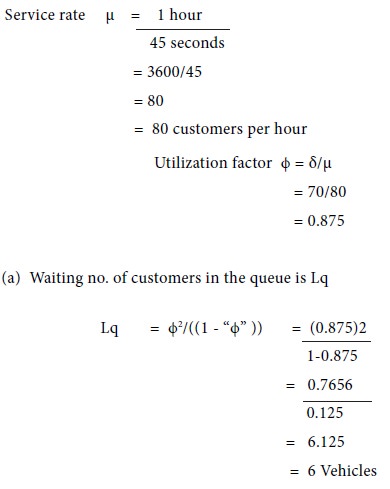
(b) Desired service time for a customer (after addition another service point) =35 seconds
The new service rate after installation of an additional service point = 1 hour/35 Seconds= 3600/35
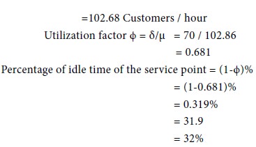
This idle time is not less than 9% which is desired by the proprietor.
In general, a queueing model can be classified into six categories using Kendall’s notation with six parameters to define a model. The parameters of this notation are as follows.
P- Arrival rate distribution i.e probability law for the arrival /inter – arrival time.
Q - Service rate distribution, i.e probability law according to which the customers are being served
R - Number of Servers (i.e., number of service points)
X - Service discipline
Y - Maximum number of customers allowed in the system
Z - Size of the calling source of the customers
A queuing model with the above parameters is denoted by the symbol (P/Q/R : X/Y/Z)
Model 1 : (M/M/1) : (GD/ ∞/ ∞) Model
This is a waiting line model with the following properties:
1. The arrival rate follows Poisson (M) distribution
2. The service rate follows Poisson distribution (M)
3. The number of servers in the system is 1
4. The service discipline is general discipline (i.e., GD)
5. Maximum number of customers allowed in the system is infinite (∞)
6. he size of the calling source is infinite (∞)
The steady state equations to obtain Pn, the probability of having n customers in the system, and the formulae for obtaining the values for Ls, Lq, Ws and Wq are as follows:
Example 1
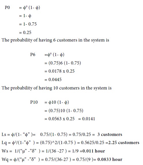
The arrival rate of customers at a petrol bunk follows a Poisson distribution with a mean of 27 per hour. The petrol bunk has only one unit of service. The service rate at the petrol bunk also follows Poisson distribution with mean of 36 per hour. Determine the following:
What is the probability of having zero customer in the system ?
What is
the probability of having 6 customers in the system ?
What is the probability
of having 10 customers in the system ?
The values of Ls, Lq, Ws and Wq
Solution
Given that the arrival rate follows Poisson distribution with mean = 27 With our notations, δ = 27 per hour
Given that the service rate follows Poisson distribution with mean = 36 Hence µ = 36 per hour
Consequently, the utilization factor ϕ = δ/µ = 27/36 = 3/4 = 0.75
The probability of having zero customer in the system is
Example 2
At one-man book binding centre, customers arrive according to Poisson distribution with mean arrival rate of 4 per hour and the book binding time is exponentially distributed with an average of 12 minutes. Find out the following:
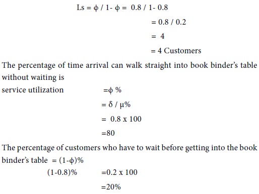
The average number of customers in the book binding centre and the average number of customers waiting for book binding.
The percentage of time arrival can walk in straight without having to wait.
The percentage of customers who have to wait before getting into the book binder’s table
Given mean arrival of customers δ = 4/60 =1/15
Mean time for server µ=1/12
Hence ϕ = δ / µ = [1/15] x 12 = 12 /15 = 0.8
The average number of customers in the system (Customers in the queue and in the book binding centre)
Example 3
A person repairing wrist watches observes that the time spent on the wrist watches has an exponential distribution with mean 20 minutes. If the wrist watches are repaired in the order in which they come in and their arrival is Poisson with an average rate of 15 for 8-hour day, what is the repairman’s expected idle time each day? On an average, how many jobs are ahead of a wrist watch just brought in?
Solution
The arrival rate δ = 15/8x60 = 1/32 units/minute
The service rate µ =
1/20 units/minute
ϕ = δ/µ
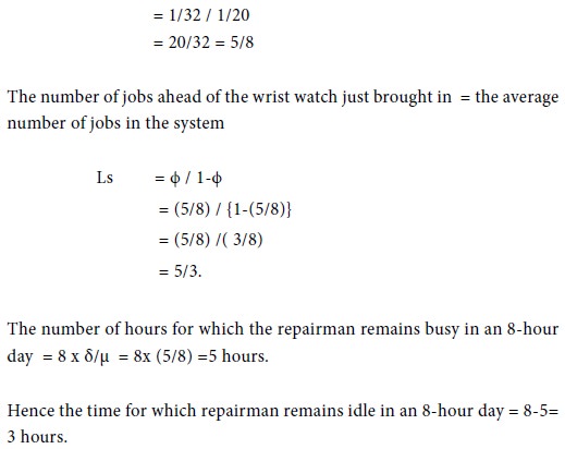
ϕ = δ/µ
Example 4
Customers are arriving at a service centre at the rate of 70 per hour. The average service time for a customer is 45 seconds. The arrival rate and service rate follow Poisson distribution. There is a complaint that the customers wait for a long duration. The proprietor of the centre is ready to consider the installation of one more service point to reduce the average time to 35 seconds if the idle time of the service point is less than 9% and the average queue length at the service point is more than 8 customers. Determine whether the installation of the second service point is worth from the point of view of the proprietor.
Solution
Arrival rate of the customers at the service centre δ =70 per hour Average service time for a customer = 45 Seconds
(b) Desired service time for a customer (after addition another service point) =35 seconds
The new service rate after installation of an additional service point = 1 hour/35 Seconds= 3600/35
This idle time is not less than 9% which is desired by the proprietor.
Hence, the installation of the second service point is not
justified since the average waiting number of customers in the queue is more than
8 but the idle time is not less than 32%.
Tags : Operations Management - Game Theory, Goal Programming & Queuing Theory
Last 30 days 2207 views