


Managerial Economics - Production Analysis
The Law Of Returns To Scale - Production Analysis
Posted On :
In the long run the fixed inputs like machinery, building and other factors will change along with the variable factors like labour, raw material etc.
The Law
Of Returns To Scale
In the long run the fixed inputs like machinery, building and other factors will change along with the variable factors like labour, raw material etc. With the equal percentage of increase in input factors various combinations of returns occur in an organization.
Returns to scale: the change in percentage output resulting from a percentage change in all the factors of production. They are increasing, constant and diminishing returns to scale.
Increasing returns to scale may arise: if the output of a firm increases more than in proportionate to an increase in all inputs. For example the input factors are increased by 50% but the output has doubled (100%).
Constant returns to scale: when all inputs are increased by a certain percentage the output increases by the same percentage. For example input factors are increased by 50% then the output has also increased by 50 percentages. Let us assume that a laptop consists of 50 components we call it as a set. In case the firm purchases 100 sets they can assemble 100 laptops but it is not possible to produce more than 100 units.
Diminishing returns to scale: when output increases in a smaller proportion than the increase in inputs it is known as diminishing return to scale. For example 50% increment in input factors lead to only 20% increment in the output.
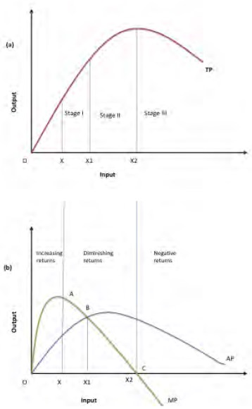
From the graph given below we can see the total production (TP) curve and the marginal production curve (MP) and average production curve (AP). It is classified into three stages; let us understand the stages in terms of returns to scale.
Stage I: The total production increased at an increasing rate. We refer to this as increasing stage where the total product, marginal product and average production are increasing.
Stage II: The total production continues to
increase but at a diminishing rate
until it reaches the next stage. Marginal product, average product are
declining but are positive. The total production is at the maximum level at the
end of the second stage with a zero marginal product.
Stage III: In this third stage total production declines and marginal product becomes negative. And the average production also started decline. Which implies that the change in input factors there is a decline in the over all production along with the average and marginal.
In the long run the fixed inputs like machinery, building and other factors will change along with the variable factors like labour, raw material etc. With the equal percentage of increase in input factors various combinations of returns occur in an organization.
Returns to scale: the change in percentage output resulting from a percentage change in all the factors of production. They are increasing, constant and diminishing returns to scale.
Increasing returns to scale may arise: if the output of a firm increases more than in proportionate to an increase in all inputs. For example the input factors are increased by 50% but the output has doubled (100%).
Constant returns to scale: when all inputs are increased by a certain percentage the output increases by the same percentage. For example input factors are increased by 50% then the output has also increased by 50 percentages. Let us assume that a laptop consists of 50 components we call it as a set. In case the firm purchases 100 sets they can assemble 100 laptops but it is not possible to produce more than 100 units.
Diminishing returns to scale: when output increases in a smaller proportion than the increase in inputs it is known as diminishing return to scale. For example 50% increment in input factors lead to only 20% increment in the output.
From the graph given below we can see the total production (TP) curve and the marginal production curve (MP) and average production curve (AP). It is classified into three stages; let us understand the stages in terms of returns to scale.
Stage I: The total production increased at an increasing rate. We refer to this as increasing stage where the total product, marginal product and average production are increasing.
Stage III: In this third stage total production declines and marginal product becomes negative. And the average production also started decline. Which implies that the change in input factors there is a decline in the over all production along with the average and marginal.
In economics, the production function with one
variable input is illustrated with the well known law of variable proportions.
(below graph) it shows the input-output relationship or production function
with one factor variable while other factors of production are kept constant.
To understand a production function with two variable inputs, it is necessary
know the concept iso-quant or
iso-product curve.
Tags : Managerial Economics - Production Analysis
Last 30 days 1730 views