


Managerial Economics - Market Structure
Monopolistic Competition - Market Structure
Posted On :
The perfect competition and monopoly are the two extreme forms. To bridge the gap the concept of monopolistic competition was developed by Edward Chamberlin.
Monopolistic
Competition
The perfect competition and monopoly are the two extreme forms. To bridge the gap the concept of monopolistic competition was developed by Edward Chamberlin. It has both the elements like many small sellers and many small buyers. There is product differentiation. Therefore close substitutes are available and at the same time it is easy to enter and easy to exit from the market. Therefore it is possible to incur loss in this market. The profit maximization for each firm, for each product depends upon the differentiation and advertising expenditure. As every firm is acting as a monopoly the same logic of monopoly is followed. Each and every firm will have their own set of cost and revenue curves and the price determination is based on the rule of MR=MC and they incur varied profits according to their market structure. But in the monopolistic competition number of monopoly competitors will be there in different levels. They monopolize in a small geographical area or a segment or a model.
The demand curve of a monopolistically competitive firm would be more elastic than that of a purely monopolistic firm. The cost function of a firm would be that there will not be any significant difference across different types of structures in the product market. Given the function, and the corresponding AR and MR curves, and the cost function, and the corresponding SAC and SMC curves, the price and output determination of a profit – maximizing monopolistically competitive firm could be as follows.
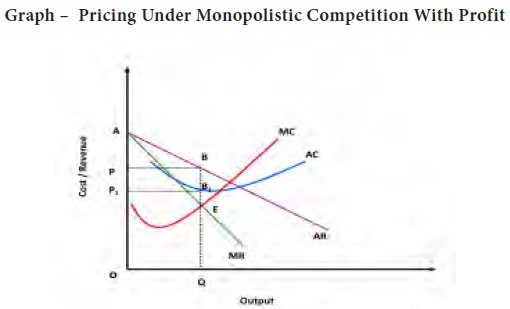
From the above graph we can
understand that under monopolistic competition firms incur profit which is PP1BB1 the pricing and profit
determination are similar to the monopoly market. MR is marginal revenue curve
AR is average revenue and demand curve. At point ‘E’ both MR and marginal cost
curve MC intersects. Based on this equilibrium the product is sold at OP price
in the market. The Average cost curve indicates that the firm has spent QB1 amount per unit but it receives
QB through its sale. Therefore the difference between the two BB1 is the profit margin which
should be multiplied with the total quantity sold OQ which gives PP1BB1 amount of profit.
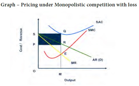
The marginal revenue curve MR and the average revenue curve AR that is the demand curve is also represented in the graph. The condition for product decision is MR=MC. The MR and MC intersect at point ‘E’ based on the equilibrium. It is decided to produce OM quantity and the price of the commodity is fixed at OP in the market. Therefore the total revenue by selling OM quantity in the market for OP price is equal to OM x OP = OPRM. But to produce OM quantity the firm has spent MQ as average cost. Therefore the total cost of production = OM x MQ = OMQS.
Therefore the profit = TR – TC
= ORPM – OMQS
= - PQRS. (Negative)
The perfect competition and monopoly are the two extreme forms. To bridge the gap the concept of monopolistic competition was developed by Edward Chamberlin. It has both the elements like many small sellers and many small buyers. There is product differentiation. Therefore close substitutes are available and at the same time it is easy to enter and easy to exit from the market. Therefore it is possible to incur loss in this market. The profit maximization for each firm, for each product depends upon the differentiation and advertising expenditure. As every firm is acting as a monopoly the same logic of monopoly is followed. Each and every firm will have their own set of cost and revenue curves and the price determination is based on the rule of MR=MC and they incur varied profits according to their market structure. But in the monopolistic competition number of monopoly competitors will be there in different levels. They monopolize in a small geographical area or a segment or a model.
The demand curve of a monopolistically competitive firm would be more elastic than that of a purely monopolistic firm. The cost function of a firm would be that there will not be any significant difference across different types of structures in the product market. Given the function, and the corresponding AR and MR curves, and the cost function, and the corresponding SAC and SMC curves, the price and output determination of a profit – maximizing monopolistically competitive firm could be as follows.
The marginal revenue curve MR and the average revenue curve AR that is the demand curve is also represented in the graph. The condition for product decision is MR=MC. The MR and MC intersect at point ‘E’ based on the equilibrium. It is decided to produce OM quantity and the price of the commodity is fixed at OP in the market. Therefore the total revenue by selling OM quantity in the market for OP price is equal to OM x OP = OPRM. But to produce OM quantity the firm has spent MQ as average cost. Therefore the total cost of production = OM x MQ = OMQS.
Therefore the profit = TR – TC
= ORPM – OMQS
= - PQRS. (Negative)
That means the cost of production
per unit is more than the average revenue earned per unit. Average revenue = MR
and the Average cost = MQ which is more than the revenue. Therefore the
difference QR is the loss per unit multiplied with OM quantity. PQRS is the
total loss to the organization.
Tags : Managerial Economics - Market Structure
Last 30 days 887 views