


Managerial Economics - Market Structure
Perfect Market - Market Structure
Posted On :
Perfect competition is a market structure characterized by a complete absence of rivalry among the individual firms.
Perfect Market
Perfect competition is a market structure characterized by a complete absence of rivalry among the individual firms. A perfectly competitive firm is one whose output is so small in relation to market volume that its output decisions have no perceptible impact on price. No single producer or consumer can have control over the price or quantity of the product.
Characteristic features of perfect market:
1. Large number of buyers and sellers
2. Homogeneous product
3. Perfect knowledge about the market
4. Ruling prices
5. Absence of transport cost
6. Perfect mobility of factors
7. Profit maximization
8. Freedom in decision making
In perfect market, the price of the commodity is determined based on the demand for and supply of the product in the market. The equilibrium price and output determination is as shown in the graph.
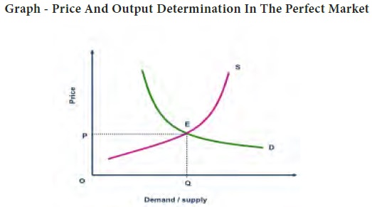
The demand curve (D) and the supply curve (S) intersect each other at a particular point which is called the equilibrium point. At the equilibrium point ‘E’ the quantity demanded and the quantity supplied are equal (that is OQ quantity of commodity is demanded and the same level is supplied etc). Based on the equilibrium the price of the commodity is fixed as OP. This is the fundamental pricing strategy followed in the perfect market.
1.
If quantity demanded is equal to
quantity supplied at a particular price then the market is in equilibrium
2.
If quantity demanded is more than
the quantity supplied then market price may not be stable. i.e., it will rise.
3.
If quantity demanded is less than
quantity supplied then market price is fixed not in a equilibrium position.
When the price at which quantity demanded is equal to quantity supplied, buyers as well as sellers are satisfied. If price is greater than the equilibrium price, some sellers would not be able to sell the commodity. So they would try to dispose the unsold stock at a lower price. Thus the price will go on declining till they get equalized (Qd = Qs). The various possible changes in Demand and supply are expressed in the following graphs to understand the price fluctuations in the market.
When the firm is producing its goods at the maximum level, the unit cost of production or managerial cost of the last item produced is the lowest. If the firm produces more than this, the managerial cost will rise. If that firm produces less than that level of output, it is not taking advantage of the economics of the large scale operation.When the firm produces largest level of output and sell at the managerial cost, it is said to be in equilibrium position.There is no temptation to produce more or produce less level of output. Likewise, when all the firms put together or the industry produces the largest amount of output at the lowest marginal cost, the industry is also said to be in the equilibrium
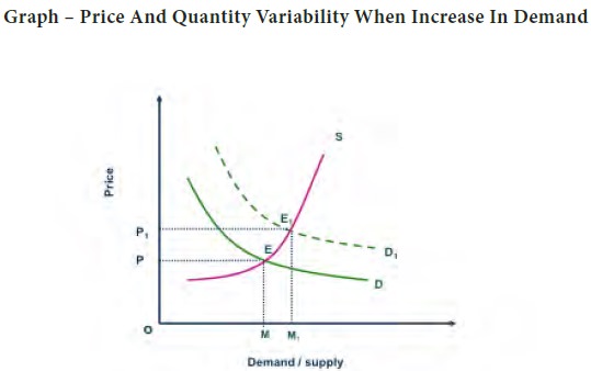
Let us assume that the demand equal to supply Qd = Qs and the equilibrium point ‘E’ determines the price as OP. In the short run the demand for the commodity increases but the supply remains the same. Then the demand curve shifts to the right and the new demand curve D1D1 is derived. The demand has increased from OM quantity to OM1. The new demand curve intersects the supply curve at the new equilibrium point ‘E1’ and the price of the commodity is increased from OP to OP1. Therefore it is clear that when demand increases without any change in supply this leads to price rise in the market.
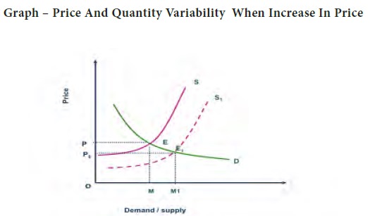
If the demand remains the same and the firm tries to supply more of the commodity, then the supply curve shifts from SS to S1S1 (Graph - below). Earlier the equilibrium point was ‘E’ and the price of the commodity was OP. Due to change in supply the equilibrium point has changed into ‘E1’ which in turn reduced the price form OP to OP0. Therefore if the firm supplies more than the demand this leads to price fall in the market.
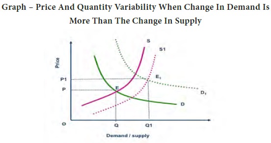
If the firm changes its supply due to increase in demand then the possible fluctuations in the price is explained below. Let us assume that the firm increased its supply 10% , the demand has also increased but not in the same proportion – it increased only 2% ( ΔQd < ΔQs). From the graph we can understand that the equilibrium point ‘E’ has changed into ‘E1’ which reduced the price of the commodity from OP to OP1.

On the other hand when there is
10% increase in the demand and the supply has increased only to 2%, the new
demand curve D1D1 and the new supply curve S1S1 intersect each other at the new equilibrium point ‘E1’.
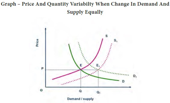
The following graph explains clearly that both the demand for the commodity and the supply increases in the same proportion (i.e. ΔQD = ΔQS).The shift in supply curve and the shift in demand curve are in the same level and the new equilibrium point ‘E1’ determines the same price OP level. There is no change in the price when the demand and supply are equal.
Perfect competition is a market structure characterized by a complete absence of rivalry among the individual firms. A perfectly competitive firm is one whose output is so small in relation to market volume that its output decisions have no perceptible impact on price. No single producer or consumer can have control over the price or quantity of the product.
Characteristic features of perfect market:
1. Large number of buyers and sellers
2. Homogeneous product
3. Perfect knowledge about the market
4. Ruling prices
5. Absence of transport cost
6. Perfect mobility of factors
7. Profit maximization
8. Freedom in decision making
In perfect market, the price of the commodity is determined based on the demand for and supply of the product in the market. The equilibrium price and output determination is as shown in the graph.
The demand curve (D) and the supply curve (S) intersect each other at a particular point which is called the equilibrium point. At the equilibrium point ‘E’ the quantity demanded and the quantity supplied are equal (that is OQ quantity of commodity is demanded and the same level is supplied etc). Based on the equilibrium the price of the commodity is fixed as OP. This is the fundamental pricing strategy followed in the perfect market.
Pricing Under Perfect Competition
Demand and supply curves can be used to analyze the equilibrium market price and the optimum output.When the price at which quantity demanded is equal to quantity supplied, buyers as well as sellers are satisfied. If price is greater than the equilibrium price, some sellers would not be able to sell the commodity. So they would try to dispose the unsold stock at a lower price. Thus the price will go on declining till they get equalized (Qd = Qs). The various possible changes in Demand and supply are expressed in the following graphs to understand the price fluctuations in the market.
When the firm is producing its goods at the maximum level, the unit cost of production or managerial cost of the last item produced is the lowest. If the firm produces more than this, the managerial cost will rise. If that firm produces less than that level of output, it is not taking advantage of the economics of the large scale operation.When the firm produces largest level of output and sell at the managerial cost, it is said to be in equilibrium position.There is no temptation to produce more or produce less level of output. Likewise, when all the firms put together or the industry produces the largest amount of output at the lowest marginal cost, the industry is also said to be in the equilibrium
Let us assume that the demand equal to supply Qd = Qs and the equilibrium point ‘E’ determines the price as OP. In the short run the demand for the commodity increases but the supply remains the same. Then the demand curve shifts to the right and the new demand curve D1D1 is derived. The demand has increased from OM quantity to OM1. The new demand curve intersects the supply curve at the new equilibrium point ‘E1’ and the price of the commodity is increased from OP to OP1. Therefore it is clear that when demand increases without any change in supply this leads to price rise in the market.
If the demand remains the same and the firm tries to supply more of the commodity, then the supply curve shifts from SS to S1S1 (Graph - below). Earlier the equilibrium point was ‘E’ and the price of the commodity was OP. Due to change in supply the equilibrium point has changed into ‘E1’ which in turn reduced the price form OP to OP0. Therefore if the firm supplies more than the demand this leads to price fall in the market.
If the firm changes its supply due to increase in demand then the possible fluctuations in the price is explained below. Let us assume that the firm increased its supply 10% , the demand has also increased but not in the same proportion – it increased only 2% ( ΔQd < ΔQs). From the graph we can understand that the equilibrium point ‘E’ has changed into ‘E1’ which reduced the price of the commodity from OP to OP1.
The price of the commodity is OP
at ‘E’ and it increases from P to P1 and becomes OP1.i.e. When the demand increases more than the supply ( ΔQd > ΔQs )
the price of the commodity will increase.
The following graph explains clearly that both the demand for the commodity and the supply increases in the same proportion (i.e. ΔQD = ΔQS).The shift in supply curve and the shift in demand curve are in the same level and the new equilibrium point ‘E1’ determines the same price OP level. There is no change in the price when the demand and supply are equal.
Tags : Managerial Economics - Market Structure
Last 30 days 1055 views