


Home | ARTS | Managerial Economics
|
Profit Maximization Under Perfect Competition - Market Structure
Managerial Economics - Market Structure
Profit Maximization Under Perfect Competition - Market Structure
Posted On :
The primary objective of any business is to maximize the profit. Profit can be increased either by increasing total revenue (TR) or by reducing the total cost (TC).
Profit
Maximization Under Perfect Competition
The primary objective of any business is to maximize the profit. Profit can be increased either by increasing total revenue (TR) or by reducing the total cost (TC). The profit is nothing but the difference between the revenue and the cost.
The total profit = TR – TC
Let us assume that whatever produced is sold in the market.
TR = Quantity sold x price
To increase the revenue, it is better to either increase the quantity sold or increase the price. Therefore while increasing the revenue or minimizing the total cost of production over a period of time with attendant economies of scale will widen the difference to gain more profit.
In perfect market, the firm’s Marginal cost, Average cost, Average revenue, Marginal revenue are equal to the price of the commodity. The cost is measured as average cost and marginal cost .When the firm is in equilibrium, producing the maximum output i.e. cost of the last item produced is known as marginal cost.The total cost divided by the number of goods produced will give the average cost. When the firm is operating in perfect market MC = AC.
In the same way the revenue available to the firm through selling goods is called as total revenue.The last item sold is the marginal revenue. The total revenue divided by the number of items sold is the average revenue and when the firm is working in the perfect market the MR shall be equal to AR. Therefore the MC = MR = AR = AC = P in the short run. The size of the plant is fixed only with the variable factors and the price is fixed by the demand and supply.
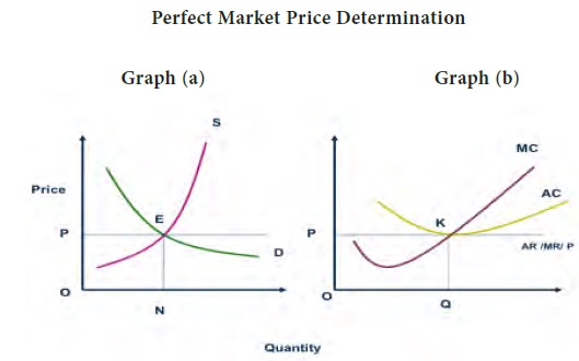
The
demand for the commodity is expressed in the demand curve (D)
and the supply (S) curve is known
as S curve. The point of intersection of the D curve and S Curve is the
equilibrium point (E) where the price is determined as OP. (Rs.10) The average
revenue per unit is also Rs.10 expressed in graph (b) along with the marginal
cost (MC) and average cost (AC) curves. The MC and AC intersect at point ‘K’
which is equal to the price OP / AR / MR. Therefore we can say that
P=AR=AC=MR=MC at this level. At this equilibrium point buyers and sellers are
satisfied with their price. The price of the commodity includes the normal
profit through the average cost. The average cost consists of implicit and
explicit costs. That means the organizers knowledge, time, idea and effort is
also considered in the cost of production. Let us assume that in the short run
the demand for the commodity increases, then the change in price and profit are
explained in the graph below.
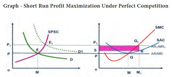
From the above graph we can understand that in the short run demand curve DD and the short period supply curve SPSC intersects at ‘E’ and the price of the commodity is determined as OP. The right side graph indicates the cost and revenue curves. The average revenue (AR) and marginal revenue (MR) are equal to the price of the commodity OP. The short period marginal cost (SMC) and short period average cost (SAC) are also depicted in the graph. The minimum average cost is selected based on the equilibrium point Q which produces optimum quantity of OM. The marginal cost curve and average cost curve intersects at the point Q that means QM amount (rupees) is spent as marginal as well as average cost. The SAC is tangential to AR/MR at this point therefore we can conclude that the price of the commodity is equal to the average cost, average revenue, marginal cost and marginal revenue ( P = AR = MR = AC = MC )
If the demand increases in the market then the new demand curve D1D1 intersects the SPSC at the new equilibrium point ‘E1’ and the price increases from OP to OP1. Therefore the average revenue also increases from AR to AR1. At this situation P1 = AR1 = MR1 but the SMC curve intersects at Q1 ie., new equilibrium point and the OM quantity has increased from OM to OM1 in the ‘X’ axis. The average cost has increased as M1R.
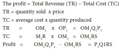
In the above graph, the shaded portion of P1Q1RS is the total profit earned by the firm in the short run but in the long run the organization will increase the production and will supply more of the commodity. Ultimately both the demand and the supply gets equalized and the short run abnormal profit becomes normal. Therefore we can conclude that even in the perfect market it is possible to earn profit in the short period.
It indicates clearly that in the short run, in any perfect market, the increase in demand will increase the profit to the businessmen. The normal profit will be there until it gets equalized with the demand i.e. new D1D1 with the increased supply of S1S1.
This economic profit attracts new firms into the industry and the entry of these new firms increases the industry supply. This increased supply pushes down the price. As price falls, all firms in the industry adjust their output levels in order to remain in profit maximizing equilibrium. New firms continue to enter the industry and price continues to fall, and existing firms continue to adjust their outputs until all economic profits are eliminated. There is no longer an incentive for the new firms to enter and the owners of all firms in the industry will earn only what they could make through their best alternatives.
Economic losses motivate some to exit (shut down) from the industry. The exit of these firms decreases industry supply. The reduction in supply pushes up market price and all the firms shall adjust their output in order to maximize their profit.
The primary objective of any business is to maximize the profit. Profit can be increased either by increasing total revenue (TR) or by reducing the total cost (TC). The profit is nothing but the difference between the revenue and the cost.
The total profit = TR – TC
Let us assume that whatever produced is sold in the market.
TR = Quantity sold x price
To increase the revenue, it is better to either increase the quantity sold or increase the price. Therefore while increasing the revenue or minimizing the total cost of production over a period of time with attendant economies of scale will widen the difference to gain more profit.
In perfect market, the firm’s Marginal cost, Average cost, Average revenue, Marginal revenue are equal to the price of the commodity. The cost is measured as average cost and marginal cost .When the firm is in equilibrium, producing the maximum output i.e. cost of the last item produced is known as marginal cost.The total cost divided by the number of goods produced will give the average cost. When the firm is operating in perfect market MC = AC.
In the same way the revenue available to the firm through selling goods is called as total revenue.The last item sold is the marginal revenue. The total revenue divided by the number of items sold is the average revenue and when the firm is working in the perfect market the MR shall be equal to AR. Therefore the MC = MR = AR = AC = P in the short run. The size of the plant is fixed only with the variable factors and the price is fixed by the demand and supply.
From the above graph we can understand that in the short run demand curve DD and the short period supply curve SPSC intersects at ‘E’ and the price of the commodity is determined as OP. The right side graph indicates the cost and revenue curves. The average revenue (AR) and marginal revenue (MR) are equal to the price of the commodity OP. The short period marginal cost (SMC) and short period average cost (SAC) are also depicted in the graph. The minimum average cost is selected based on the equilibrium point Q which produces optimum quantity of OM. The marginal cost curve and average cost curve intersects at the point Q that means QM amount (rupees) is spent as marginal as well as average cost. The SAC is tangential to AR/MR at this point therefore we can conclude that the price of the commodity is equal to the average cost, average revenue, marginal cost and marginal revenue ( P = AR = MR = AC = MC )
If the demand increases in the market then the new demand curve D1D1 intersects the SPSC at the new equilibrium point ‘E1’ and the price increases from OP to OP1. Therefore the average revenue also increases from AR to AR1. At this situation P1 = AR1 = MR1 but the SMC curve intersects at Q1 ie., new equilibrium point and the OM quantity has increased from OM to OM1 in the ‘X’ axis. The average cost has increased as M1R.
In the above graph, the shaded portion of P1Q1RS is the total profit earned by the firm in the short run but in the long run the organization will increase the production and will supply more of the commodity. Ultimately both the demand and the supply gets equalized and the short run abnormal profit becomes normal. Therefore we can conclude that even in the perfect market it is possible to earn profit in the short period.
It indicates clearly that in the short run, in any perfect market, the increase in demand will increase the profit to the businessmen. The normal profit will be there until it gets equalized with the demand i.e. new D1D1 with the increased supply of S1S1.
This economic profit attracts new firms into the industry and the entry of these new firms increases the industry supply. This increased supply pushes down the price. As price falls, all firms in the industry adjust their output levels in order to remain in profit maximizing equilibrium. New firms continue to enter the industry and price continues to fall, and existing firms continue to adjust their outputs until all economic profits are eliminated. There is no longer an incentive for the new firms to enter and the owners of all firms in the industry will earn only what they could make through their best alternatives.
Economic losses motivate some to exit (shut down) from the industry. The exit of these firms decreases industry supply. The reduction in supply pushes up market price and all the firms shall adjust their output in order to maximize their profit.
Tags : Managerial Economics - Market Structure
Last 30 days 1663 views